Chapter 28
Optimization
return to the Course index
previous | next
Optimization Methods
Notes on Optimization with Boomer
When setting up an optimization with boomer upper and lower limits are required for each adjustable, fitted parameter. With good data and model you might start with lower limits half or a tenth of the initial estimate and upper limits twice or tens time the initial estimate. For apparent volumes of distribution a value of zero during optimization will produce a divide by zero error so an non-zero lower limit should be entered. For rate constants a lower limit of zero might be quite useful. You should start with relatively narrow limits and expand them only when appropriate and a warning of 'close to limits' is displayed in the output. With more difficult problems it might be useful to constrain the more well estimated parameters with very tight limits, recognizing that you will hits limits on this run but may get useful initial values to use on the next run with more liberal estimates. The upper and lower limits are hard limits, rather like the walls of a box. There are not constraints until a limit is hit.
You should also consider using different initial estimates to avoid acceptance of convergence to a local minimum. The simplex or simplex-DGN method described below can be useful in helping to find a global minimum. You should also careful review the output plots for evidence of local, non-global minima.
The damping Gauss-Newton method provides progress output.
 Loop =     1
 Damp =     1
 P ( 1) =       .5808
 P ( 2) =       .1106
 P ( 3) =       2.101
 P ( 4) =       39.64
 WSS =        55.5363


 Loop =     2
 Damp =     1
 P ( 1) =       .4375
 P ( 2) =       .1319
 P ( 3) =       2.199
 P ( 4) =       42.54
 WSS =        10.6959
Each iteration is represented as a loop number. Damp numbers higher than 2 or 3 indicate that the surface may be irregular.
The Nelder-Mead (Simplex) method also provides progress output.
 Loop   1 -
   1>   717.5      2>   643.2      3>   386.5      4>   973.2      5>   797.9
 Loop   2 -
   1>   717.5      2>   643.2      3>   386.5      4>   127.4      5>   797.9
 Loop   3 -
   1>   717.5      2>   643.2      3>   386.5      4>   127.4      5>   120.6
 Loop   4 -
   1>   58.02      2>   643.2      3>   386.5      4>   127.4      5>   120.6
 Loop   5 -
   1>   58.02      2>   38.82      3>   386.5      4>   127.4      5>   120.6
From line to line there should be one value, the highest, WSS reduced from the previous line.
If selecting the Simplex or Simplex->Damping GN method a convergence criteria (PC) must be entered. If the Gauss-Newton, Damping Gauss-Newton, or Marquardt method is selected a step-size (DT value) must entered as well. When editing a .BAT file there is one more line with these methods. The DT value specifies the step-size used to create the partial differentials used in the optimization process (Jacobian). In both cases (PC and DT) the default values usually work well.
 FITTING METHODS

 0) Gauss-Newton
 1) Damping Gauss-Newton
 2) Marquardt
 3) Simplex
 4) Simplex->Damping GN

 Enter Choice (0-4)      4

 Enter PC for convergence (0.00001)      .000
or
 FITTING METHODS

 0) Gauss-Newton
 1) Damping Gauss-Newton
 2) Marquardt
 3) Simplex
 4) Simplex->Damping GN

 Enter Choice (0-4)      1

 Enter DT for Jacobian (0.001)      .000

 Enter PC for convergence (0.00001)      .000
The first three methods are numerically intensive, relative to the simplex method, thus there may be occasions when poorly defined calculations may produce 'fatal' errors, for example divide by zero or other math error. Better initial estimates or use of the less numerically intensive simplex method may be useful.
Repeated Runs using the Simplex Method
Another advantage of the simplex method as implemented in Boomer is that once the initial estimates (first point on the simplex) are specified the other points on the simplex are randomly generated. This means that each time a problem is run a different initial simplex is used and effectively different initial estimates are used with each run. This can be set-up automatically by adding a line after the first and entering the number of runs to be attempted. Consider,
Boomer Batch File
    5                             wls,bayes,sim,irwls,sim+error,grid
    1                             Screen, diskfile
outfname
    1                             Parameter type
Dose
   100.0                          Parameter value
If the -2 on the last line is replaced with a -4 and followed, on a new line, with the name of the xxxx.BAT file without the .BAT, Boomer will rerun the .BAT file repeatedly using a different initial simplex each time until the user stops the program with a control-C (or similar).
Boomer Batch File
20
    5                             wls,bayes,sim,irwls,sim+error,grid
    1                             Screen, diskfile
outfname
    1                             Parameter type
Dose
   100.0                          Parameter value
The .OUT file will now contain the results of multiple runs and the WSS (and other results) from each run can be examined. Typically, hopefully, there will be a majority of runs that converge to the same 'global' minimum with only a few that might stops with higher WSS values.
Notes on Optimization with Phoenix™
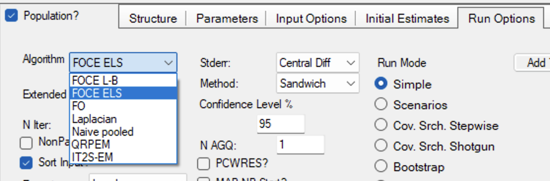
The optimization methods avaialble in Phoenix™ include:
- FOCE Lindstrom-Bates (FOCE L-B) FOCE ELS
- FO engine
- Naive pooled engine
For population data this method treats all the data as from a single subject.
- Laplacian
- QRPEM
- Adaptive Gaussian quadrature
- NonParametric engine
The optimization method is specified on the Run Options tab.
More details can be found in the Maximum Likelihood Models User's Guide.
With Phoenix™, the parameters are transformed so upper and lower limits are normally not required. In some limited cases such as negative "best-fit" values for clearance or rate constant a lower limit of zero may be needed. When using the QRPEM or Naive pooled methods a lower limit of zero is set by the program.
This page was last modified: Sunday, 28th Jul 2024 at 5:08 pm
Privacy Statement - 25 May 2018
Material on this website should be used for Educational or Self-Study Purposes Only
Copyright © 2001 - 2026 David W. A. Bourne (david@boomer.org)
 | Drug Structures
A game to aid recognizing drug structures
See how many structures you can name before you run out of lives |

|