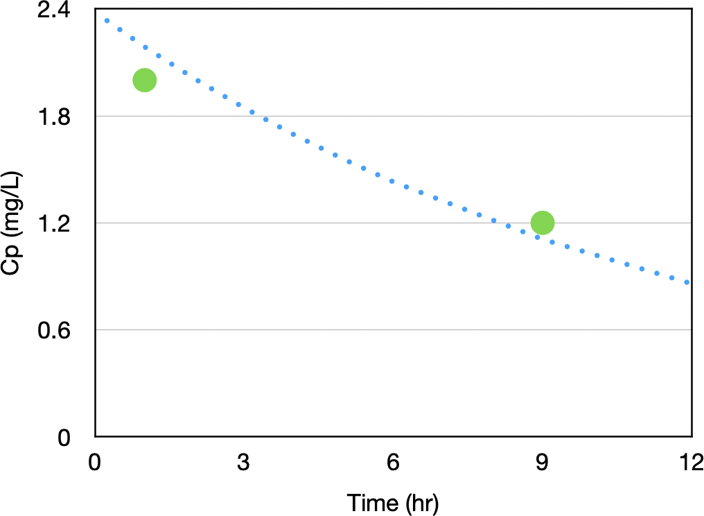
Figure 29.9.1 Simulated Concentration Time Data with Two Data Points
return to the Course index
previous | next
Figure 29.9.1 Simulated Concentration Time Data with Two Data Points
Combining these data points with our prior information about the pharmacokinetic model and model parameters we can perform a Bayesian analysis of the data.
 Enter type# for parameter  1 (-5 to 51) 1
 Enter parameter name Dose
 Enter Dose value 100
 0) fixed, 1) adjustable, 2) single dependence
                    or 3) double dependence 0
 Enter component to receive dose 1
 Enter component for F-dependence ( 1 to - 1 or 0 for no dependence)

 Input summary for Dose                 (type  1)

     Fixed value is    100.0
     Dose/initial amount added to     1

 Enter 0 if happy with input, 1 if not, 2 to start over

 Enter -3 to see choices, -1 or -4 (save model) to exit this section
 Enter type# for parameter  2 (-5 to 51)  2
 Enter parameter name kel
 Enter kel value 0.085
 0) fixed, 1) adjustable, 2) single dependence
                    or 3) double dependence 1
 Enter lower limit 0
 Enter upper limit 1
 Enter mean parameter value 0.085
 Enter standard deviation 0.025
 Enter component to receive flux 0
 Enter component to lose flux 1

 Input summary for kel                  (type  2)

     Initial value   0.8500E-01 float between    0.000     and    1.000
     Population mean   0.8500E-01 with std-dev   0.2500E-01
     Transfer from     1 to     0

 Enter 0 if happy with input, 1 if not, 2 to start over

 Enter -3 to see choices, -1 or -4 (save model) to exit this section
 Enter type# for parameter  3 (-5 to 51)  18
 Enter parameter name V
 Enter V value 42
 0) fixed, 1) adjustable, 2) single dependence
                    or 3) double dependence 1
 Enter lower limit 1
 Enter upper limit 100
 Enter mean parameter value 42
 Enter standard deviation 17
 Enter data set (line) number 1
 Enter line description Cp
 Enter component number (0 for obs x) 1

 Input summary for V                    (type 18)

     Initial value    42.00     float between    1.000     and    100.0
     Population mean    42.00     with std-dev    17.00
     Component     1 added to line     1

 Enter 0 if happy with input, 1 if not, 2 to start over

 Enter -3 to see choices, -1 or -4 (save model) to exit this section
 Enter type# for parameter  4 (-5 to 51)  -1
The results of this analysis are shown in Figure 22.3.4
                    ** FINAL PARAMETER VALUES ***

  #  Name                  Value       S.D.       C.V. %  Lower <-Limit-> Upper
              Population mean         S.D.        (Weight)  Weighted residual

  1) kel                   0.84658E-01  0.208E-02   2.5       0.0       1.0
                       0.8500E-01   0.2500E-01     40.00      -0.1369E-01
  2) V                      42.175       1.25       3.0       1.0      0.10E+03
                        42.00        17.00        0.5882E-01   0.1030E-01

 Final WSS =   0.143082E-01  R^2 =    1.000     Corr. Coeff =    1.000
 AIC =   -4.49385            AICc =    0.00000
 Log likelihood =   2.10     Schwarz Criteria =   -7.10755
 R^2 and R - jp1      1.000         1.000
 R^2 and R - jp2     0.8809        0.9386
 RMSE =     0.1425     or          8.371 % RMSE
 MAE  =     0.1359     ME =     0.4267E-01

 Model and Parameter Definition

  #  Name                    Value       Type From To     Dep  Start Stop

  1) Dose                =   100.0        1    0    1       0    0    0
  2) kel                 =  0.8466E-01    2    1    0       0    0    0
  3) V                   =   42.18       18    1    1       0    0    0

 Data for Cp :-

 DATA #   Time       Observed      Calculated    (Weight)  Weighted residual

     1    1.000       2.00000       2.17860      0.500000     -0.892979E-01
     2    9.000       1.20000       1.10674      0.833333      0.777201E-01
iBook and pdf versions of this material and other PK material is available
Copyright © 2001-2022 David W. A. Bourne (david@boomer.org)