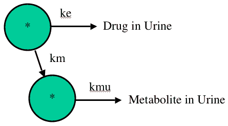
Figure 31.4.1 Diagram representing and IV Administration, One Compartment Model with Metabolism
return to the Course index
previous | next
Figure 31.4.1 Diagram representing and IV Administration, One Compartment Model with Metabolism
Data were simulated for drug and metabolite concentrations are shown in Table 31.4.1
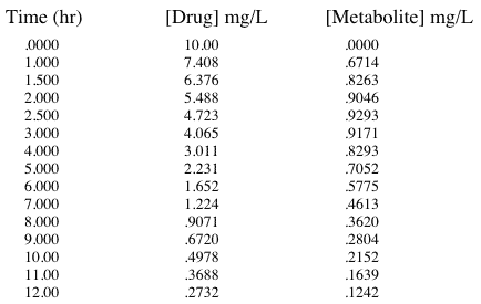
Table 31.4.1 Data Simulated for Cp and Cm
The data were then fitted to the model in Figure 31.4.1 using Boomer.
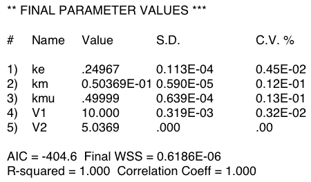
Table 31.4.2 Output from Boomer
Table 31.4.2 shows just one result from fitting the data in Table 31.4.1. Note that the CV% values look good for most of the parameters. This generally indicates a good fit and well defined parameters. However, the value of zero for V2 (= Vm) is not a good sign. The real problem becomes apparent when the model is fit multiple times with the same data. Now we see a variety of values for ke, km and Vm. Curiously if the best-fit ke and km values are plotted it can be seen that they fall on a line indicating a common value of kel (= ke + km).
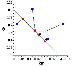
Figure 31.4.2 Plot of ke versus km
The blue squares represent the initial values used for each fit and the red circle represents the final, best-fit, value. Note that all the red circles fall on a straight line representing the value of kel (= ke + km). This indicates the neither ke nor km are identifiable but does suggest that kel is identifiable.
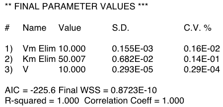
Figure 31.4.3 Output from Boomer - 500 mg Dose
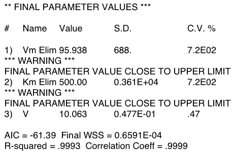
Figure 31.4.4 Output from Boomer - 5 mg Dose
Notice that the CV% for the low dose are quite large (720%) indicating that Vm (=Vmax) and Km are not identifiable with these low dose data. Note also that the parameters have hit reasonable upper limits. Increasing the limits resulted in the values increasing to the new limits. The value for the parameter CV% using the high dose data are much better. The final parameter values for all three estimated parameters are close to the starting values. This indicates that if data as good as the simulated data were available then these parameters would be identifiable.
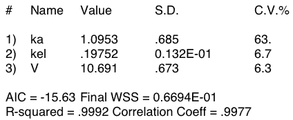
Figure 31.4.5 Output from Boomer - Oral Administration with Missing Early Data Points
Notice the high value for CV% for the ka parameter value compared with the CV% for kel and V. Clearly ka is not well defined.
iBook and pdf versions of this material and other PK material is available
Copyright © 2001-2022 David W. A. Bourne (david@boomer.org)