PHAR 4634 - Chapter 19 Page 5

Apparent volumes of distribution

The concentration of drug in the body is determined not only by the rate constant values but also by the apparent volume of distribution. In the case of the two compartment model a number of volume terms can been defined.

V₁

The apparent volume of the central compartment, V₁ or V_c, can be calculated as:-

Equation XIX-2 Apparent Volume of Central Compartment

This parameter is important because it allows the calculation of the highest plasma concentration or Cp⁰ after an IV bolus administration. This concentration may result in transient toxicity. V₁ can also be used in dose calculations.

V_area ( = V_ß)

V_area or V_ß is defined as:-

= V_ß

Equation XIX-3 Apparent Volume, V_area

Because of the relationship with clearance and and with V₁ and kel this parameter is quite useful in dosing calculations. This parameter can be readily calculated via AUC and values from the 'raw' data and is therefore commonly quoted.

V_extrap

V_extrap calculated as:-

Equation XIX-4 Apparent Volume, Extrapolated

This is the volume value calculated if the distribution phase is ignored. Generally not very useful. However, you may see it used. You will be using this if the distribution phase is ignored. (That is, it is the V calculated using a one compartment model with a two compartment drug).

V_ss

V_ss, V steady state defined as:-

Equation XIX-5 Apparent Volume, Steady State

This term relates the total amount of drug in the body at 'steady state' with the concentration in plasma or blood

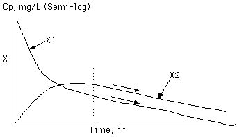
Figure XIX-8, Plot of X1 (Plasma) and X2 (Tissue) Compartment Concentrations, Showing ÔSteady StateÕ with Both Lines Parallel

The relationship between volume terms is that:-

V_extrap > V_area > V_ss > V₁

And for a one compartment model the values for all these parameters are equal.

Example Calculation

As an example we can look at the data in the table below.

Table XIX-1 Two Compartment Pharmacokinetics

Time (hr) Concentration (mg/L) Cplate (mg/L) Residual (mg/L)

0.5 20.6 8.8 11.8

1 13.4 7.8 5.6

2 7.3 6.1 1.2

3 5.0 4.7 0.3

4 3.7 3.7 -

6 2.2

8 1.4

10 0.82

12 0.50

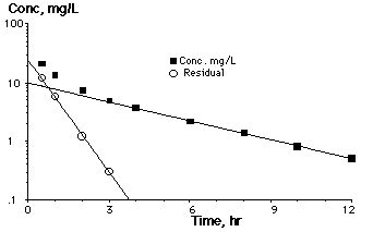
Figure XIX-9 Plot of Cp versus Time Illustrating the Method of Residuals

The first two columns are the time and plasma concentration which may be collected after IV bolus administration of 500 mg of drug. These data are plotted (n) in Figure XIX-9, above. At longer times, after 4 hours, out to 12 hours the data appears to follow a straight line on semi- log graph paper. Since > this terminal line is described by B * e^{- *t}.

Following it back to t = 0 gives B = 10 mg/L. From the slope of the line [ = 0.25 hr^-1. Cp^late values at early times are shown in column 3 and the residual in column 4. The residual values are plotted (o) also giving a value of A = 25 mg/L and = 1.51 hr^-1 Note that / = 6, thus these values should be fairly accurate.

B = 10 mg/L, = (ln 10 - ln 0.5)/12 = 2.996/12 = 0.25 hr^-1

A = 25 mg/L, = (ln 25 - ln 0.27)/3 = 4.528/3 = 1.51 hr^-1

Therefore Cp = 25 * e^{-1.51 * t} + 10 * e^{-0.25 * t}

We can now calculate the microconstants.

= 0.61 hr-1