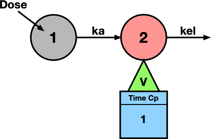
Figure 8.3.1 Diagram Representing a One Compartment Model after Oral Administration
| Boomer Manual and Download | ||||
| PharmPK Listserv and other PK Resources | ||||
| Previous Page | Course Index | Next Page | ||
Figure 8.3.1 Diagram Representing a One Compartment Model after Oral Administration
The next step is to convert the parts in the model to parameters from the Boomer parameter toolbox. This could be done by notation on the diagram above or by preparing a table of parameter types. Currently the available parameter types within Boomer include:
MODEL Definition and Parameter Entry       * Allowed Parameter Types *

 -5) read model         -3) display choices      -2) display parameters

  0) Time interrupt      1) Dose/initial amount   2) First order rate
  3) Zero order          4-5) Vm and Km of Michaelis-Menten
  6) Added constant      7) Kappa-Reciprocal volume
  8-10) C = a * EXP(-b * (X-c))
 11-13) Emax (Hill) Eq with Ec(50%) & S term     14) Second order rate
 15-17) Physiological Model Parameters (Q, V, and R)
 18) Apparent volume of distribution   19) Dummy parameter for double dependence
 20-22) C = a * SIN(2 * pi * (X - c)/b)

 Special Functions for First-order Rate Constants
 23-24) k = a * X + b                  25-27) k = a * EXP(-b * (X - c))
 28-30) k = a * SIN(2 * pi * (X - c)/b)
 31,32-33) dAt/dt = - k * V * Cf (Saturable Protein Binding)
 34-36) k * (1 - Imax * C/(IC(50%) + C)) Inhibition  0 or 1st order
 37-39) k * (1 + Smax * C/(SC(50%) + C)) Stimulation 0 or 1st order
 40) Uniform [-1 to 1] and 41) Normal [-3 to 3] Probability
 42) Switch parameter                  43) Clone component
 44-47) Four parameter logistic model  48-51) Four parameter Weibull model
The model in Figure 8.3.1 has a dose (type 1), two first order rate constants (a type 2 parameter) and an apparent volume of distribution (type 18). These can represented in tabular form before starting the program.
| Parameter Name | Parameter Type | Flow Direction | Value | Limits |
|---|---|---|---|---|
| Dose | 1 Dose/Initial Value | Into 1 | 100 | Fixed |
| ka | 2 First Order | From 1 to 2 | 1.0 | 0.0 - 10.0 |
| kel | 2 First Order | From 2 to 0 | 0.1 | 0.0 - 1.0 |
| V | 18 Volume | From 2 to Data Set 1 | 15 | 1.0 - 100.0 |
Table 8.3.1 Parameter Types and Values for the Model in Figure 8.3.1
Now it is time to start the program. Boomer is a menu driven program. That is, once started the program will present the user with a set sequence of menu choices. Initially the user will select input and output options and 'Normal Fitting' for nonlinear regression analysis. The model is described to the program through a series of questions and prompts.
 Enter type# for parameter  1 (-5 to 51)      1
 Enter parameter name  Dose
 Enter Dose value     100.0
 0) fixed, 1) adjustable, 2) single dependence
                    or 3) double dependence      0
 Enter component to receive dose      1
 Enter component for F-dependence ( 1 to - 1 or 0 for no dependence)      0

 Input summary for Dose                 (type  1)

     Fixed value is    100.0
     Dose/initial amount added to     1

 Enter 0 if happy with input, 1 if not, 2 to start over      0

 Enter -3 to see choices, -1 or -4 (save model) to exit this section
 Enter type# for parameter  2 (-5 to 51)       2
 Enter parameter name  ka
 Enter ka value     1.000
 0) fixed, 1) adjustable, 2) single dependence
                    or 3) double dependence      1
 Enter lower limit     0.000
 Enter upper limit     10.00
 Enter component to receive flux      2
 Enter component to lose flux      1

 Input summary for ka                   (type  2)

     Initial value    1.000     float between    0.000     and    10.00
     Transfer from     1 to     2

 Enter 0 if happy with input, 1 if not, 2 to start over      0

 Enter -3 to see choices, -1 or -4 (save model) to exit this section
 Enter type# for parameter  3 (-5 to 51)       2
 Enter parameter name  kel
 Enter kel value    0.1000
 0) fixed, 1) adjustable, 2) single dependence
                    or 3) double dependence      1
 Enter lower limit     0.000
 Enter upper limit     1.000
 Enter component to receive flux      0
 Enter component to lose flux      2

 Input summary for kel                  (type  2)

     Initial value   0.1000     float between    0.000     and    1.000
     Transfer from     2 to     0

 Enter 0 if happy with input, 1 if not, 2 to start over      0

 Enter -3 to see choices, -1 or -4 (save model) to exit this section
 Enter type# for parameter  4 (-5 to 51)      18
 Enter parameter name  V
 Enter V value     15.00
 0) fixed, 1) adjustable, 2) single dependence
                    or 3) double dependence      1
 Enter lower limit     1.000
 Enter upper limit     100.0
 Enter data set (line) number      1
 Enter line description  Cp
 Enter component number (0 for obs x)      2

 Input summary for V                    (type 18)

     Initial value    15.00     float between    1.000     and    100.0
     Component     2 added to line     1


 Enter 0 if happy with input, 1 if not, 2 to start over      0

 Enter -3 to see choices, -1 or -4 (save model) to exit this section
 Enter type# for parameter  5 (-5 to 51)      -1
Fitting and optimization algorithms are selected.
Method of Numerical Integration

 0) Classical 4th order Runge-Kutta
 1) Runge-Kutta-Gill
 2) Fehlberg RKF45
 3) Adams Predictor-Corrector with DIFSUB
 4) Gears method for stiff equations with PEDERV
 5) Gears method without PEDERV

 Enter choice (0-5) 2

 Enter Relative error term for
     Numerical integration (0.0001)

 Enter Absolute error term for
     Numerical integration (0.0001)

 FITTING METHODS

 0) Gauss-Newton
 1) Damping Gauss-Newton
 2) Marquardt
 3) Simplex
 4) Simplex->Damping GN

 Enter Choice (0-4) 4

 Enter PC for convergence (0.00001)
Finally the data and weighting schemes are entered.
Enter data from

 0) Disk file      2) ...including weights
 1) Keyboard       3) ...including weights

 Enter Choice (0-3) 1

 Enter data for Cp
      Enter x-value (time) = -1 to finish data entry


 X-value (time) 0.0
 Y-value (concentration) 0.0

 X-value (time) 0.5
 Y-value (concentration) 1.89

 X-value (time) 1
 Y-value (concentration) 2.9

 X-value (time) 1.5
 Y-value (concentration) 3.38

 X-value (time) 2
 Y-value (concentration) 3.56

 X-value (time) 3
 Y-value (concentration) 3.46

 X-value (time) 4
 Y-value (concentration) 3.12

 X-value (time) 6
 Y-value (concentration) 2.38

 X-value (time) 9
 Y-value (concentration) 1.52

 X-value (time) 12
 Y-value (concentration) 0.97

 X-value (time) 18
 Y-value (concentration) 0.40

 X-value (time) 24
 Y-value (concentration) 0.16

 X-value (time) -1

...

 Weighting function entry for Cp

 0) Equal weights
 1) Weight by 1/Cp(i)
 2) Weight by 1/Cp(i)^2
 3) Weight by 1/a*Cp(i)^b
 4) Weight by 1/(a + b*Cp(i)^c)
 5) Weight by 1/((a+b*Cp(i)^c)*d^(tn-ti))

 Data weight as a function of Cp(Obs)

 Enter choice (0-5) 2
Refer to the Boomer manual for more detail. Boomer (Reference https://www.boomer.org/boomer/BoomerManual.pdf)
iBook and pdf versions of this material and other PK material is available
Copyright © 2001-2022 David W. A. Bourne (david@boomer.org)