
Figure 8.5.1 Importing Data in a csv File
| Boomer Manual and Download | ||||
| PharmPK Listserv and other PK Resources | ||||
| Previous Page | Course Index | Next Page | ||
Figure 8.5.1 Importing Data in a csv File
This csv file included a header row with units. Check Has a header row and Has units in column header. Note the comma is selected as the Field Delimiter. Select the Data Set > Send To > Modeling > Least-Squares Regression Models > PK Model.

Figure 8.5.2 Choosing the Model and Mapping the Data
Under the Setup Tab choose Main to choose the PK model to be use and map the data columns to the correct heading. Time to Time and Concentration to Concentration. Here we have data collected after oral administration. Model 3 represents a one compartment model with no lag time and elimination is by a first order process. A diagram illustrating the model is shown in the right panel. If Modeling > Maximum Likelihood Models had been chosen the model could be represented graphically or textually for more flexibility.
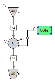
Figure 8.5.3 Graphical Representation of a One Compartment Model after Oral Administration
Aa represents the amount in the dose compartment, A1 is the central compartment and A0 the elimination (urine) compartment. CObs is the observed concentration calculated as A1/V.

Figure 8.5.4 Textual Representation of a One Compartment Model after Oral Administration (Phoenix Modeling Language [PLM])
The two deriv and the one urinecpt equation represent the differential equations for the A1, A0 and Aa components of the model. Concentration, C is defined as A1/V. The stparm equations map the typical (e.g. tvV) parameter values to the parameter values (V). The typical values are used in population pharmacokinetic analysis. The fixef equations provide initial estimates with lower and upper bounds. Here the bounds are not defined and the initial estimates are set to 1 before being determined during the curve stripping step.
The dose can be entered using the Setup > Dosing tab with Use Internal Worksheet checked. Data weighting can be chosen from the Weighting/Dosing Option tab below.

Figure 8.5.5 Dose and Weighting Options
With a simple linear model we can have WinNonlin generate the initial parameter estimates using a curve stripping technique. Alternately the user can enter initial estimates after selecting User Supplied Initial Parameter Values.
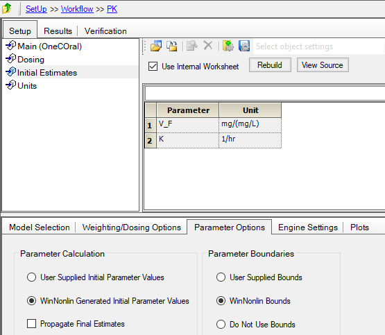
Figure 8.5.6 Parameter Options
We are now ready to execute the PK model by clicking on the green arrow at the top.
Refer to the Help menu for more details. The Maximum Likelihood Models option is very flexible and a more complete description is beyond the scope of this page.
Screenshots are from Phoenix WinNonlin version 8.3.1 March 2021.
iBook and pdf versions of this material and other PK material is available
Copyright © 2001-2022 David W. A. Bourne (david@boomer.org)