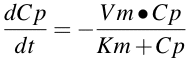
Equation 21.3.1 Rate of Change of Drug Concentration with Time
return to the Course index
previous | next
Equation 21.3.1 Rate of Change of Drug Concentration with Time
Keeping track of units becomes even more important with non linear kinetics. In Equation 21.3.1 the units for Vm are amount.volume-1.time-1 for example mg.L-1.day-1. Another approach is to derive the equation for the rate of change of drug amount with time.
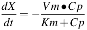
Equation 21.3.2 Rate of Change of Drug Amount with Time
Equation 21.3.2 looks the same as Equation 21.3.1. The difference is the dX/dt on the left and the units for Vm on the right. The units for Vm are the same as dX/dt, i.e. amount.time-1 for example mg/day. Note the units for Vm are the same as the units for the differential term on the left hand side of Equations 21.3.1 and 2. The Cp units cancel top and bottom.
Dividing the rate of elimination (metabolism) by the drug concentration provides a value for the drug clearance.
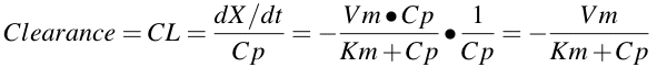
Equation 21.3.3 Non linear Equation for Clearance
Notice that Equation 21.3.3 includes a concentration term on the right hand side (in the denominator). Clearance is not constant but varies with concentration. As the concentration increases we would expect the clearance to decrease. Calculations based on an assumption of constant clearance, such as the calculation of AUC are no longer valid. A simple increasing of dose becomes an adventure. No longer can we increase the dose by some fraction, for example 25%, and expect the concentration to increase by the same fraction. The calculations are more complex and must be done carefully. The superposition principle can no longer be applied to concentration.
It is not possible to integrate Equation 21.3.1 explicitly but by looking at low and high concentrations we can get some idea of the plasma concentration versus time curve.

where the Vm/Km is a constant term and the whole equation now looks like that for first order elimination, with Vm/Km a pseudo first order rate constant for metabolism, km.
Therefore at low plasma concentrations we would expect first order kinetics. Remember, this is the usual situation for most drugs. That is Km is usually larger than the therapeutic plasma concentrations.
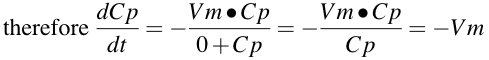
and we now have zero order elimination of drug, that is the rate of elimination is INDEPENDENT of drug concentration (remaining to be eliminated). At high plasma concentrations we have zero order or concentration independent kinetics.

Figure 21.3.1 Linear Plot of Rate of Elimination Versus Concentration with Vm and Km

Figure 21.3.2 Linear Plot of Cp Versus Time Showing High Cp and Low Cp - Zero Order and First Order Elimination
Click on the figure to view the interactive graph
In Figure 21.3.2 at high Cp, in the zero order part, the slope is fairly constant (straight line on linear graph paper) and steeper, that is, the rate of elimination is faster than at lower concentrations. [However, the apparent rate constant is lower. This is easier to see on the semi-log graph in Figure 21.3.3.]
At higher concentrations the slope is equal to -Vm. At lower concentrations we see an exponential decline in plasma concentration such as we see with first order elimination.
On semi-log graph paper we can see that in the zero order region the slope is more shallow, thus the apparent rate constant is lower. The straight line at lower concentrations is indicative of first order kinetics.

Figure 21.3.3 Semi-Log Plot of Cp Versus Time Showing High Cp and Low Cp
Click on the figure to view the interactive graph
Another way to use or look at Figure 21.3.3 is to consider the slope of the line as a measure of a psuedo or apparent first order rate constant, k'. If we start with Equation 21.3.2 since this includes Vm with the more usual units of amount/time (mg/day) we can derive equation Eq 21.3.3 for this psuedo first order rate constant.
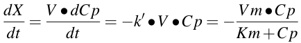
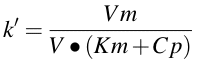
Equation 21.3.4 Psuedo First Order Rate Constant
As for clearance described earlier (Equation 21.3.4) this pseudo rate of elimination changes with concentration. As the concentration increases the elimination process slows down. We can take this one step further by looking at a 'half-life' for the elimination.
Equation 21.3.5 Psuedo Half life for Elimination
Earlier when we talked about linear kinetics we talked about the time it takes to get to steady state concentrations. With linear kinetics this time was independent of concentration and could be calculated as 3, 4 or 5 half-lives. With non-linear kinetics, this time will increase with concentration just as this psuedo half-life increases with concentration. This is very important later when we use steady state concentrations to make parameter estimates. If we don't wait long enough our determination of steady state concentration will be in error and so will the parameter estimates. This time to steady state might change from a few days to weeks as the dose is increased.
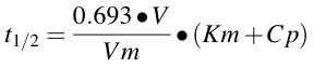
Averaging Equation 21.3.1 over a dosing interval at steady state where the dose is equal to the drug metabolized during the interval leads to Equation 21.3.6
Equation 21.3.6 Dose Required to Achieve an Average Concentration
Rearrangement of Equation 21.3.6 to solve for Cpaverage can be used to illustrate the problem of arbitrarily increasing the dose for a drug that exhibits non linear, Michaelis-Menten (MM), kinetics.
Equation 21.3.7 Average Concentration at Steady State
The presence of saturation kinetics can be quite important when high doses of certain drugs are given, or in the case of over-dose. In the case of high dose administration the effective elimination rate constant is reduced and the drug will accumulate excessively if saturation kinetics are not understood.
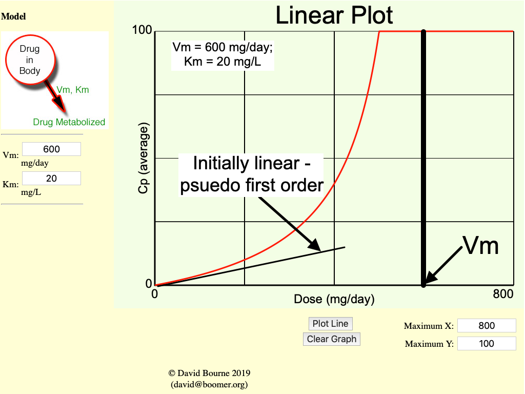
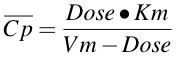
Figure 21.3.4 Linear Plot of Cpaverage Versus Dose Per Day
Click on the figure to view the interactive graph
Phenytoin is an example of a drug which commonly has a Km value within or below the therapeutic range. The average Km value is about 4 mg/L. The normally effective plasma concentrations for phenytoin are between 10 and 20 mg/L. Therefore it is quite possible for patients to be overdosed due to drug accumulation. At low concentration the apparent half-life is about 12 hours, whereas at higher concentration it may well be much greater than 24 hours. Dosing every 12 hours, the normal half-life, could rapidly lead to dangerous accumulation. At concentrations above 20 mg/L elimination maybe very slow in some patients. Dropping for example from 25 to 23 mg/L in 24 hours, whereas normally you would expect it to drop from 25 -> 12.5 -> 6 mg/L in 24 hours. Typical Vm values are 300 to 700 mg/day. These are the maximum amounts of drug which can be eliminated by these patients per day. Giving doses approaching these values or higher would cause very dangerous accumulation of drug. Figure 21.3.4 is a plot of Cpaverage versus dose calculated using Equation 21.3.7.

Equation 21.3.8 Rate of Change of Drug Amount with Time after Oral Administration
At higher concentrations the slope is equal to -Vm. At lower concentrations we see an exponential decline in plasma concentration such as we see with first order elimination.
On semi-log graph paper we can see that in the zero order region the slope is more shallow, thus the apparent rate constant is lower. The straight line at lower concentrations is indicative of first order kinetics.
Figure 21.3.5 Linear Plot of Cp Versus Time after Oral Administration Showing High Cp and Low Cp - Zero Order and First Order Elimination
Click on the figure to view the interactive graph
Material on this website should be used for Educational or Self-Study Purposes Only
Copyright © 2001 - 2026 David W. A. Bourne (david@boomer.org)
 | Pharmacy Math Part Two A selection of Pharmacy Math Problems |
 |