Optimal Sampling
Graphical Approach
One Compartment - IV Bolus
Let's start with the one compartment pharmacokinetic model after an intravenous (IV) bolus. The equation concentration versus time is given by Equation 21.2.1.

Equation 21.2.1 Concentration versus Time - One Compartment IV Bolus
The question is: What are the best times to sample for kel and V.
Using the graphical approach the steps are:
- Simulate data using the known model and the expected parameter values
- Adjust one parameter (at a time) by a small amount (± 1, 5, 10%) in both directions
- Plot ΔCp/ΔParameter Value versus Time
- Determine the time of maximum change
Starting with the concentration versus time curve, Figure 21.2.1.
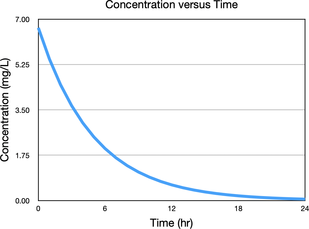
Figure 21.2.1 Concentration versus Time after IV Bolus Administration
Now vary the value of kel higher and lower while holding V constant and repeat the calculation as seen in Figure 21.2.2.
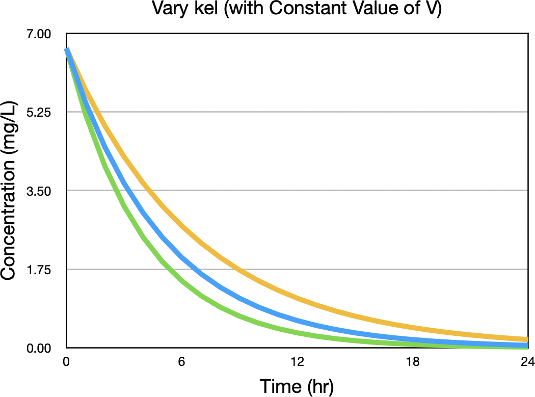
Figure 21.2.2 Concentration versus Time after an IV Bolus with three values of kel
Notice the values of Cp are close to equal early in the plot and at the end, near 24 hours. The next step is to calculate the difference between the upper and lower curves, dividing the differences by the difference in kel. Note this difference is greater towards the middle, maybe left of middle in Figure 21.2.2. The following plot represents ΔCp/Δkel versus time. The time of maximum ratio is indicated at time five hours. Here kel was 0.2 hr-1.
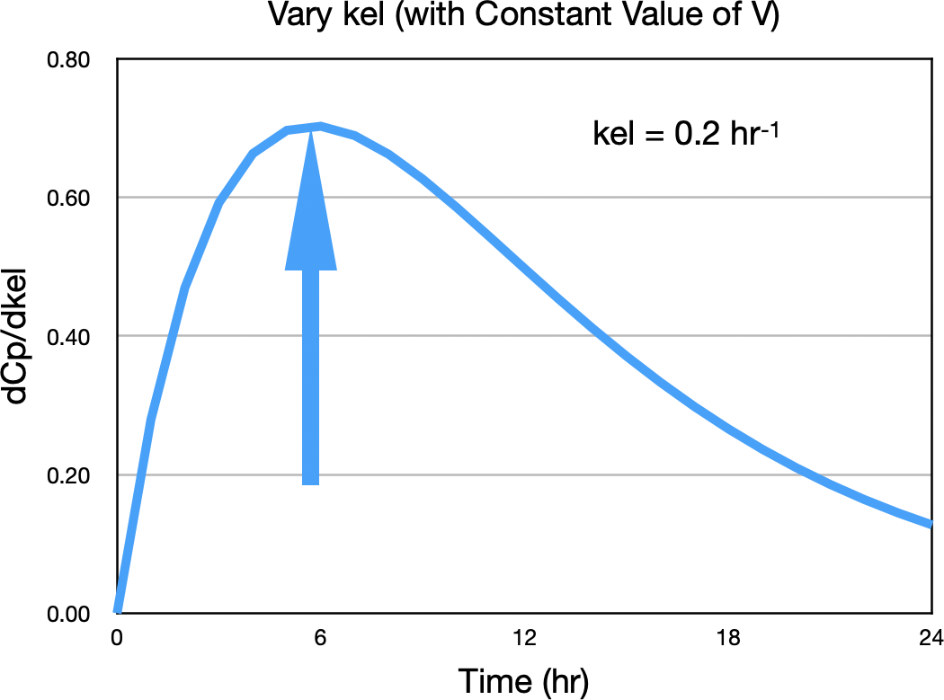
Figure 21.2.3 ΔCp/Δkel versus Time
Now we can do the same thing for V, the apparent volume of distribution. Plotting concentration versus time with values of V above and below the expected value of 15 L gives the concentrations in Figure 21.2.4.
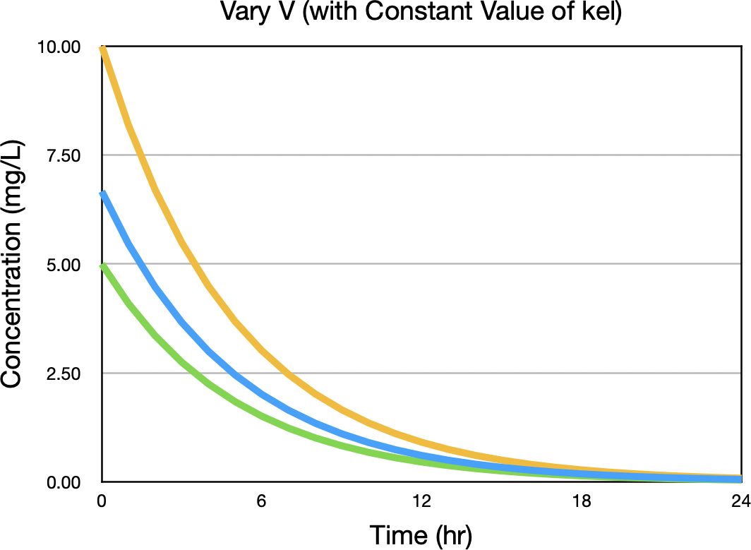
Figure 21.2.4 Concentration versus Time after an IV Bolus with three values of V
Notice the biggest difference between concentration values is near zero time. Figure 21.2.5 confirms this observation.
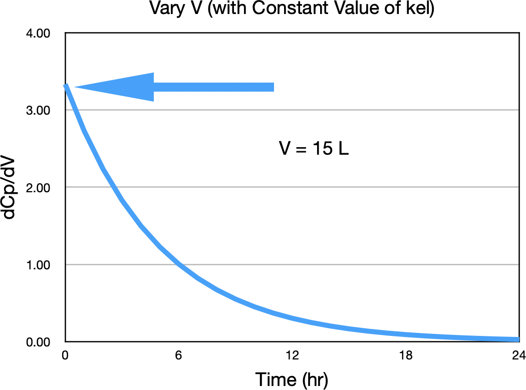
Figure 21.2.5 ΔCp/ΔV versus Time
This indicates that the best time to sample for V is close to time zero. That is, as early as possible in the sampling schedule.
This approach can be used for any parameter of a pharmacokinetic model with know or expected values for the parameters.
One Compartment - Oral
Another example might be to determine the best times to sample for three parameters on the one compartment model after oral administration, i.e. kel, ka and V. The equation concentration versus time is given by Equation 21.2.1.

Equation 21.2.2 Concentration versus Time - One Compartment Oral
For this model the question is: What are the best times to sample for kel, ka and V.
Using the method described above, the steps are:
- Simulate data using the known model and the expected parameter values
- Adjust one parameter (at a time) by a small amount (± 1, 5, 10%) in both directions
- Plot ΔCp/ΔParameter Value versus Time
- Determine the time of maximum change
Best Sample Time for kel
Starting with the concentration versus time curve, Figure 21.2.6.
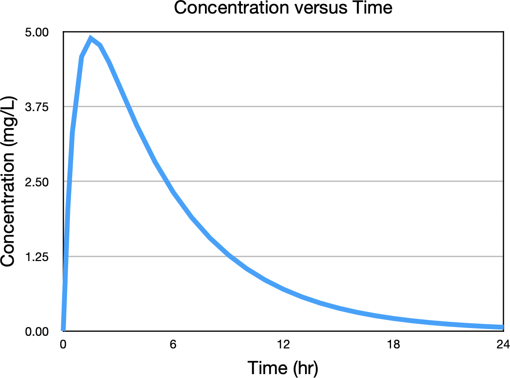
Figure 21.2.6 Concentration versus Time after Oral Administration
Now vary the value of kel higher and lower while holding ka and V constant and repeat the calculation as seen in Figure 21.2.7.
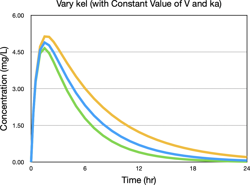
Figure 21.2.7 Concentration versus Time after Oral Administration with three values of kel
The biggest difference between concentration values is after the peak, around six hours. Figure 21.2.8.
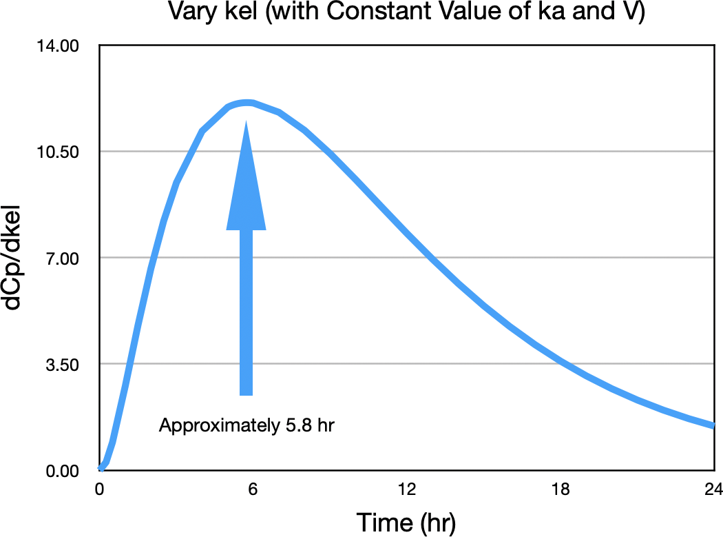
Figure 21.2.8 ΔCp/Δkel versus Time
This indicates that the best time to sample for kel is approximately 5.8 hr.
Now we can do the same thing for ka, the first order absorption rate constant. Plotting concentration versus time with values of ka above and below the expected value of 1.5 hr-1 gives the concentrations in Figure 21.2.9.
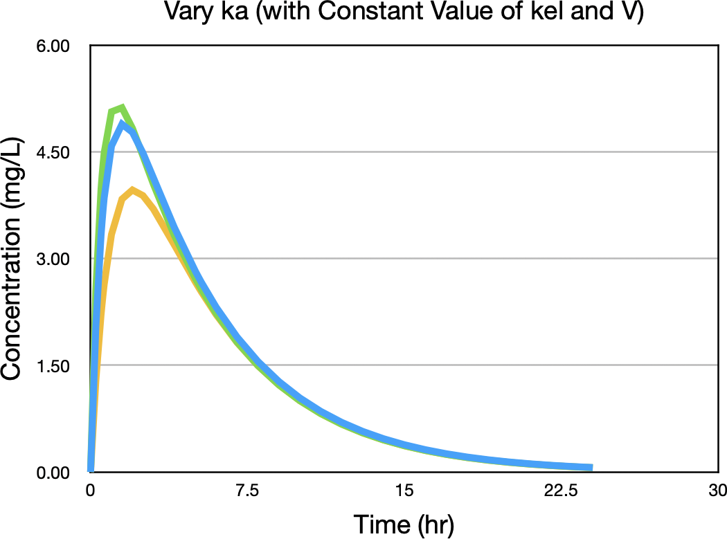
Figure 21.2.9 Concentration versus Time after Oral Administration with three values of ka
Notice the biggest difference between concentration values is near the peak concentration. Figure 21.2.10 confirms this observation.
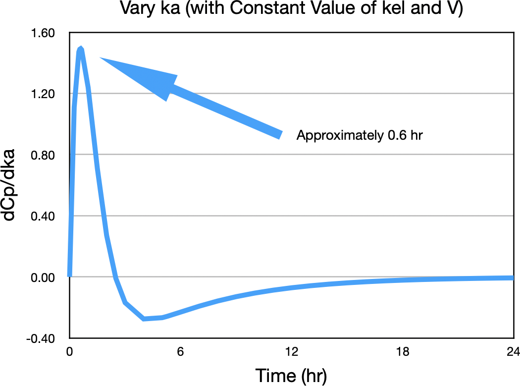
Figure 21.2.10 ΔCp/Δka versus Time
This indicates that the best time to sample for ka is early, approximately 0.6 hour.
Finally we can do the same thing for V. Plotting concentration versus time with values of V above and below the expected value of 15 L gives the concentrations in Figure 21.2.11.
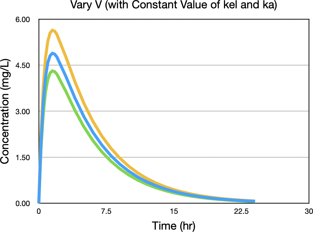
Figure 21.2.11 Concentration versus Time after Oral Administration with three values of ka
Notice the biggest difference between concentration values is near the peak concentration. Figure 21.2.12 confirms this observation.
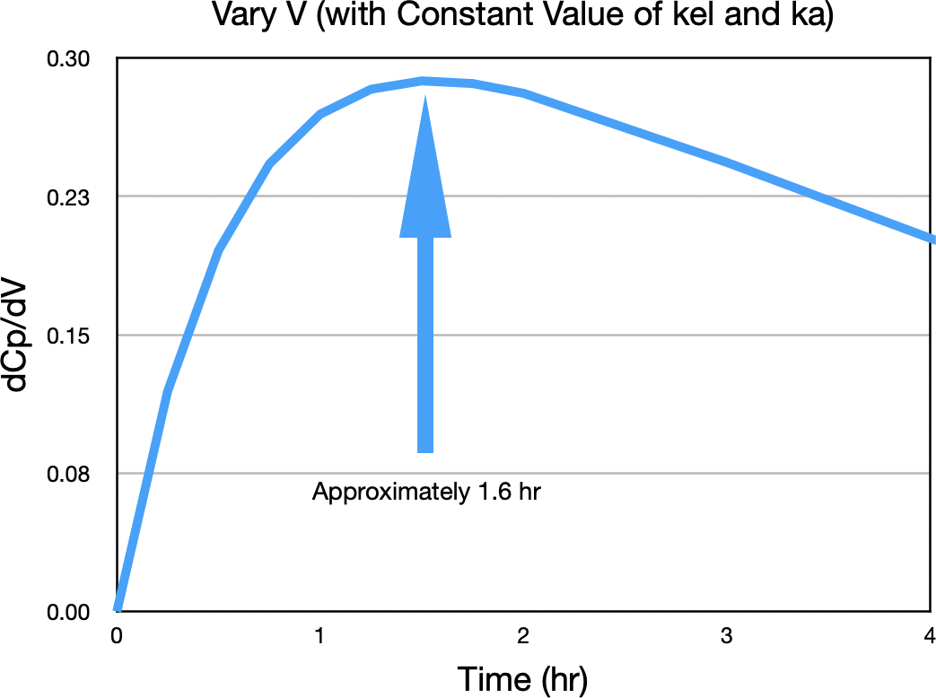
Figure 21.2.12 ΔCp/ΔV versus Time
This indicates that the best time to sample for V is near the peak concentration, approximately 1.6 hour.
return to the Course index
This page was last modified: Sunday, 28th Jul 2024 at 5:04 pm
Privacy Statement - 25 May 2018
iBook and pdf versions of this material and other PK material is available
Copyright © 2001-2022 David W. A. Bourne (david@boomer.org)