Chapter 25 Non-Linear Regression Analysis of Population Data

return to the Course index
previous | next

Analysis using of Population Data using Phoenix™ NLME

During the development of new drug entities (NDE) the manufacturer will study the disposition of the drug in numerous volunteers healthy and otherwise. The early, Phase I studies are typically conducted in healthy volunteers with the objective of determining the disposition characteristics of the NDE. These studies usually involve the collection of numerous blood and other samples from each subject. The data analysis techniques described earlier in this course may be quite useful for these studies. Later studies during Phase III involve the administration of the NDE to numerous patients who may be expected to have some therapeutic benefit from the NDE. These subjects may provide a wide range of covariates such as age, weight, sex, genetic characteristics, co-administration of other drugs and various clinical or pathological conditions. In these studies the protocol may provide for the collection of only one or two blood samples during various dosage regimens. It is difficult to analyze data separately to determine good estimate of the pharmacokinetic parameters. Fortunately these studies provide data from a large number of subjects and there are a number of computer programs which are capable of analyzing these data simultaneously.

One of these population pharmacokinetic (PopPK) computer programs is Phoenix™ NLME. Other PopPK may be found here. NLME will allow the analyst to include data from many subjects in one analysis and provides estimates of the best-fit pharmacokinetic parameter values and estimates of their variability (standard deviation or variance) between the subject as well as relationships with covariate values. The output from these analyses may be useful in the Bayesian estimate of clinical pharmacokinetic data as described earlier. The PopPK approach can also be used in cases of data rich sources, such as bioavailability studies, or sparse data information that might be available post-marketing during therapeutic drug monitoring.

A Typical (Initial) Workflow

After starting the program a new Project can be selected from the File Menu.

Figure 25.5.1 A new NLME Project

Use File > Import to select a suitable data file, maybe a .csv file. This one includes a Dose column.

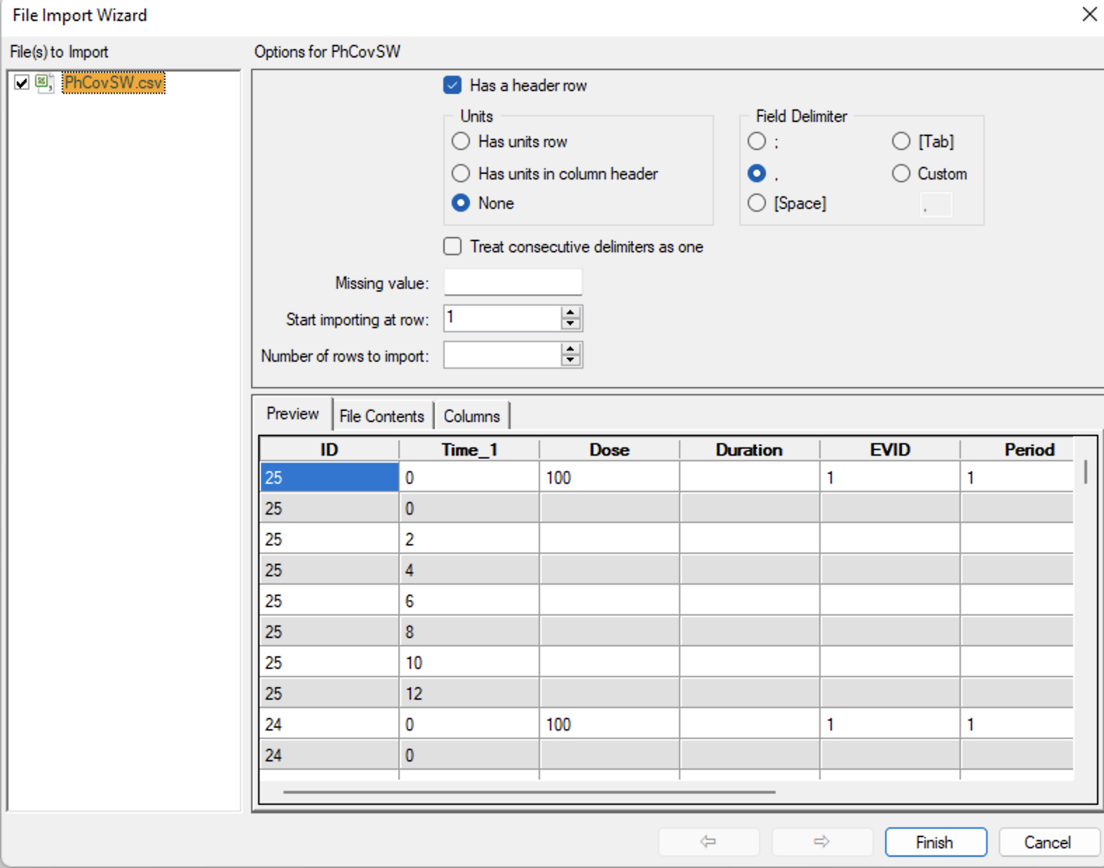
Figure 25.5.2 Import Data from a CSV File

Once the data file has been imported we can create a XY plot. Control-click on the Data file and Send to > Plotting > XY Plot. Map the X and Y to Time and CObs and Group by ID.

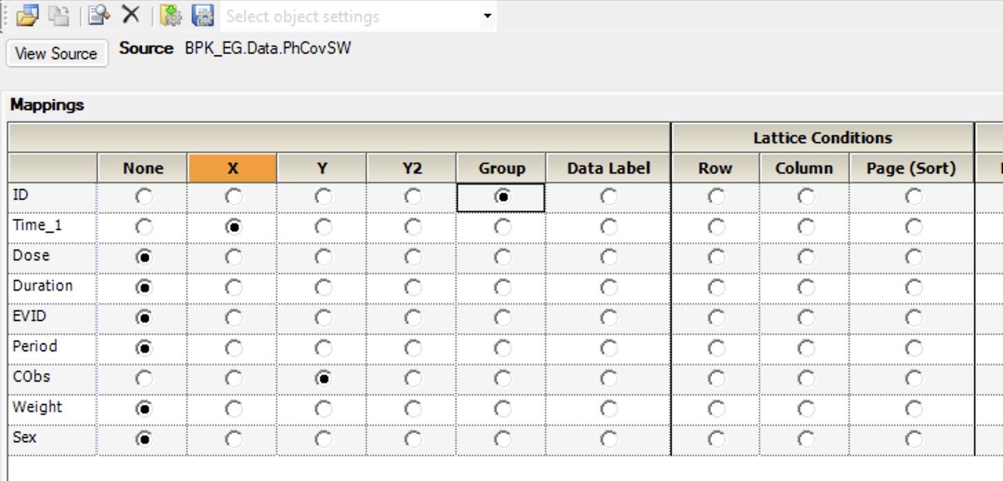
Figure 25.5.3 Map the X and Y values

Executing this object produces the first graphical look at the data.

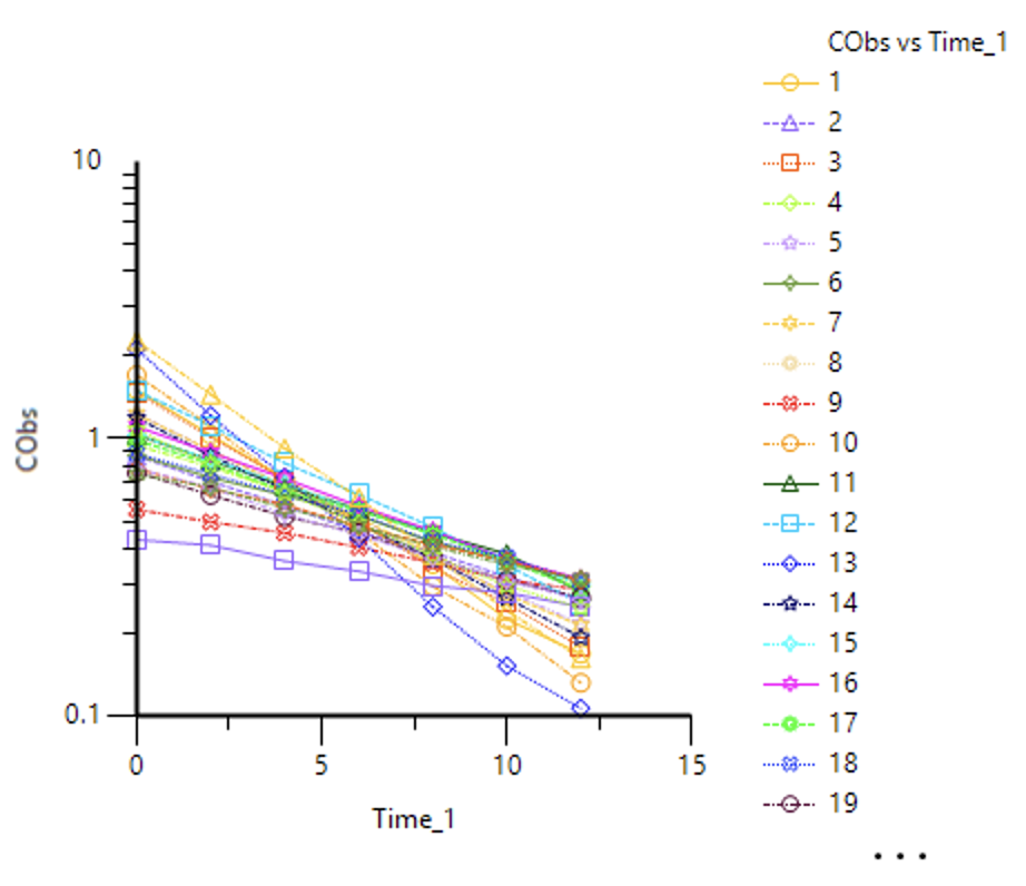
Figure 25.5.4 Semi-log plot of the Data

On this semi-log plot the data after an IV bolus appear to follow a straight line for each subject. Let try a simple one compartment model using kel and V as parameters. Control-click on the Data file and Send To... > Modeling > Maximum Likelihood Models. Map the Time_1 and Cobs values to Time and CObs. ID to ID. Dose to A1.

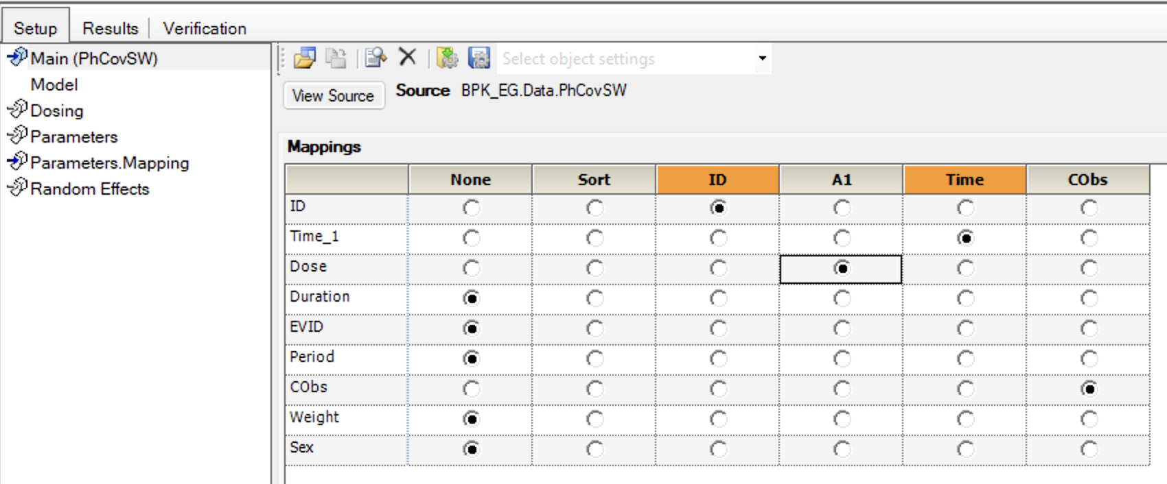
Figure 25.5.5 Mapping ID, Time and CObs

Down below check Population? Under the Structure Tab select Type: PK, Parameterization: Micro, Num Compartments: 1 and Residual Error: Multiplicative with the default Stdev: 0.1.

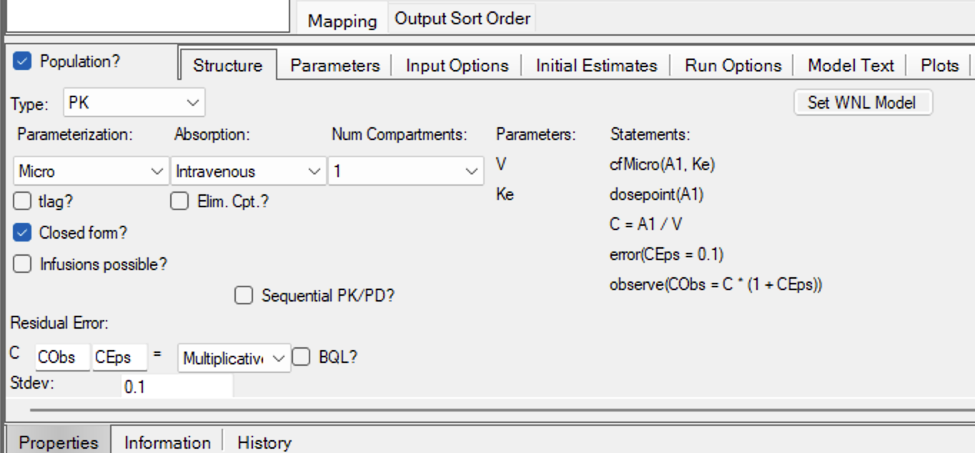
Figure 25.5.6 Structure Tab Entries

Under the Parameters: Fixed Effects Tab enter 100 for tvV and 0.1 for tvKe.

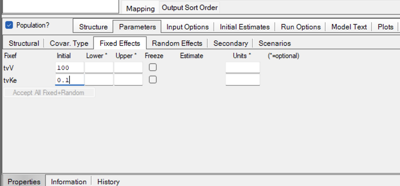
Figure 25.5.7 Enter Initial Estimates

Executing this object provides tabular and graphical output.

Figure 25.5.8 Overall Output

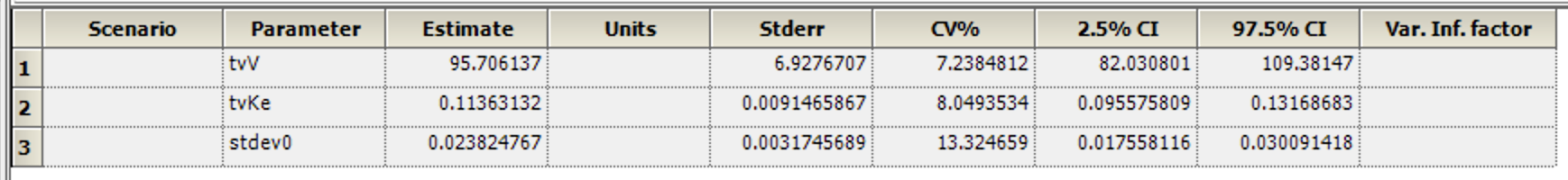
Figure 25.5.9 Best-fit Theta Values

Not too bad with no covariates included in this model.

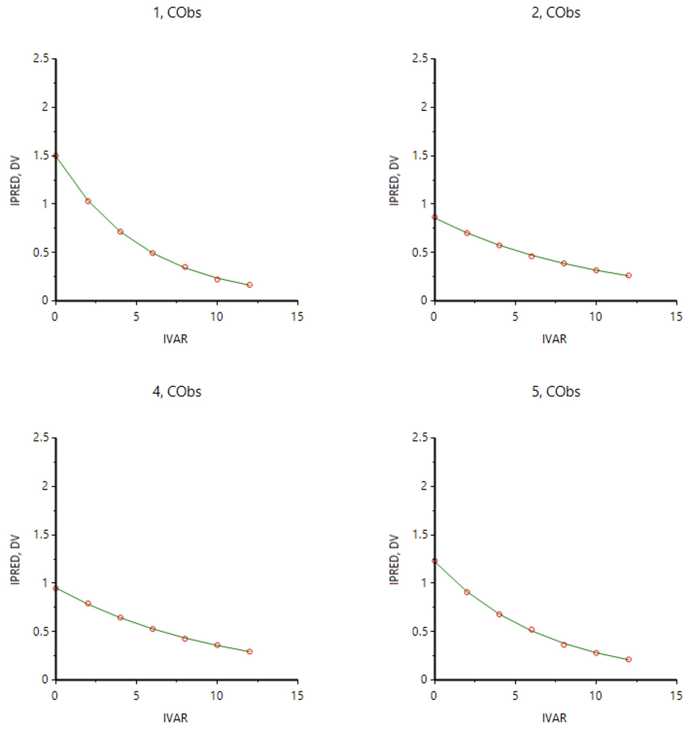
Figure 25.5.10 A few of the Observed (DV-CObs) and Calculated (IPRED) versus Time (IVAR) Plots

And a plot of Conditional Weighted Residuals (CWRES) versus Time (TAD)

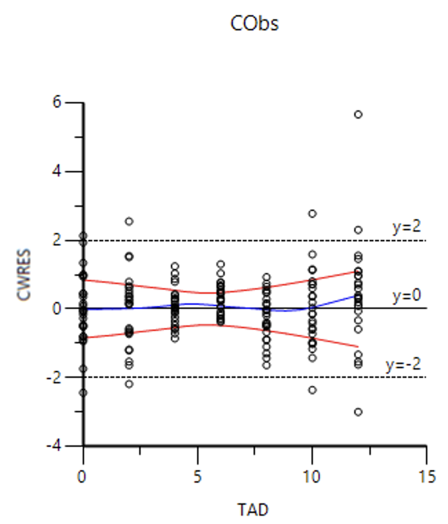
Figure 25.5.11

This is just the start. Maybe try a two compartment model. Consider different weighting schemes although multiplicative error is a good place to start. Covariates, weight and sex, could be considered for inclusion in the model.

This page was last modified: Sunday, 28th Jul 2024 at 5:06 pm

Privacy Statement - 25 May 2018

Material on this website should be used for Educational or Self-Study Purposes Only

Bird Count
An iPhone app that facilitates the geotagging of Bird Count stops
and the return to the same stops during the next
and subsequent Bird Count sessions