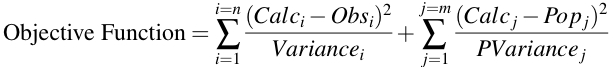
Equation 25.4.1 Objective Function for Bayesian Optimization
return to the Course index
previous | next
Equation 25.4.1 Objective Function for Bayesian Optimization
Note the use of variance instead of weight in this objective function, Equation 25.4.1. Realistic values for the data variance (and thus weight) must be balanced with variance of each population parameter. The inclusion of patient data and population data provides the ability to estimate parameters in the patient for improved drug regimen recommendations.
In this section we will briefly describe how to set up one non-linear regression program, Boomer.
| Parameter | Mean Value | Standard Deviation | Variance |
| V (L) | 30.1 | 4.2 | 17.6 |
| Clearance (L/hr) | 3.61 | 1.47 | 2.16 |
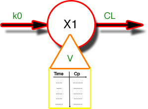
Figure 25.4.1 Another Diagram Illustrating a One Compartment Model with an IV Infusion
After a dose of 1000 mg/hr for 30min (500 mg IV) samples were collected at 1 hr and 9hr after the start of the infusion. These samples were assayed and found to contain 15.6 and 5.8 mg/L, respectively. Assay standard deviations were estimated to be 5% of the value measured. These patient data and the population parameters from Table 25.4.1 were analyzed with Boomer using the Bayesian method. Figure 25.4.2 illustrates the resulting 'best-fit' to these two data points.
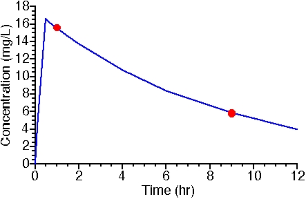
Figure 25.4.2 Linear Plot of Concentration versus Time
METHOD OF ANALYSIS 0) Normal fitting 1) Bayesian 2) Simulation only 3) Iterative Reweighted Least Squares 4) Simulation with random error 5) Grid Search -5) To perform Monte Carlo run (Only once at the start of BAT file) -4) To perform multi-run (End of BAT file only) -3) To run random number test subroutine -2) To close (or open) .BAT file -1) To finish Enter choice (-3 to 5) 1 |
Figure 25.4.3 Specifying the Bayesian Analysis Method
Model and Parameter Definition # Name Value Type From To Dep Start Stop 1) CL = 3.613 19 0 0 0 0 0 2) Vd = 29.33 19 0 0 0 0 0 3) kel = 0.1232 2 1 0 7001002 0 0 4) V = 29.33 18 1 1 1002000 0 0 5) Duration = 0.5000 0 0 0 0 0 0 6) k0 = 1000. 3 0 1 0 0 1 |
Figure 25.4.4 Model Specification from the .OUT File
Weighting function entry for [Theophylline] 0) Equal weights 1) Weight by 1/Cp(i) 2) Weight by 1/Cp(i)^2 3) Weight by 1/a*Cp(i)^b 4) Weight by 1/(a + b*Cp(i)^c) 5) Weight by 1/((a+b*Cp(i)^c)*d^(tn-ti)) Data weight as a function of Cp(Obs) Enter choice (0-5) 3 Enter a value 0.0025 Enter b value 2 |
Figure 25.4.5 Specifying the Weight for the Data Points by Equation
(Section 1)
 ** FINAL OUTPUT FROM Boomer (v3.1.5) **      26 July 2005 ---  2:21:06 pm

 Title:  Bayesian Fit to Data
 Input: From Keyboard
 Output:  To Fig2206.OUT
 Data for [Theophylline]  came from keyboard (or ?.BAT)
 Fitting algorithm: DAMPING-GAUSS/SIMPLEX
 Weighting for [Theophylline]  by 1/a*Cp(Obs )^b
      With a = 0.2500E-02 and b =  2.000
 Bayesian Fitting to data:
 Numerical integration method: 2) Fehlberg RKF45
          with  1 de(s)
 With relative error   0.1000E-03
 With absolute error   0.1000E-03
 DT =   0.1000E-02     PC =   0.1000E-04 Loops =     1
 Damping =     1

(Section 2)
                    ** FINAL PARAMETER VALUES ***

  #  Name                  Value       S.D.       C.V. %  Lower <-Limit-> Upper
              Population mean         S.D.        (Weight)  Weighted residual

  1) CL                     3.6134      0.904E-02  0.25       1.0       10.
                        3.610        1.470        0.6803       0.2309E-02
  2) Vd                     29.330      0.822E-01  0.28       1.0      0.10E+03
                        30.10        4.200        0.2381      -0.1833

 Final WSS =   0.385777E-01 R^2 =    1.000     Corr. Coeff =    1.000
 AIC =   -2.51016     Log likelihood =   1.11     Schwartz Criteria =   -5.12387
 R and R^2 - jp1     1.0000        1.0000
 R and R^2 - jp2     1.0000        1.0000


(Section 3)
 Model and Parameter Definition

  #  Name                    Value       Type From To     Dep  Start Stop

  1) CL                  =   3.613       19    0    0       0    0    0
  2) Vd                  =   29.33       19    0    0       0    0    0
  3) kel                 =  0.1232        2    1    0 7001002    0    0
  4) V                   =   29.33       18    1    1 1002000    0    0
  5) Duration            =  0.5000        0    0    0       0    0    0
  6) k0                  =   1000.        3    0    1       0    0    1

(Section 4)
 Data for [Theophylline]  :-

 DATA #   Time       Observed      Calculated    (Weight)  Weighted residual

     1    0.000       0.00000       0.00000       0.00000       0.00000
     2   0.1250       0.00000       4.22917       0.00000       0.00000
     3   0.2500       0.00000       8.39372       0.00000       0.00000
     4   0.3750       0.00000       12.4946       0.00000       0.00000
     5   0.5000       0.00000       16.5329       0.00000       0.00000
     6   0.7500       0.00000       16.0314       0.00000       0.00000
     7    1.000       15.6000       15.5452       1.28205      0.702675E-01
     8    1.500       0.00000       14.6165       0.00000       0.00000
     9    2.000       0.00000       13.7433       0.00000       0.00000
    10    4.000       0.00000       10.7420       0.00000       0.00000
    11    6.000       0.00000       8.39608       0.00000       0.00000
    12    9.000       5.80000       5.80182       3.44828     -0.625972E-02
    13    12.00       0.00000       4.00914       0.00000       0.00000

     WSS for data set  1 =   0.4977E-02
               R^2 =    1.000     Corr. Coeff. =    1.000
 R and R^2 - jp1     1.0000        1.0000
 R and R^2 - jp2     1.0000        1.0000
|
Figure 25.4.6 Tabular and Statistical Output
(Section 1) Preliminary Output describing the input/output details, the fitting (optimization) algorithm, integration method and weighting scheme.
(Section 2) Best-fit parameter values with statistical information are provided. The parameter CV values, the WSS, AIC and other values provide information about the model and how well the data have been fit to the model.
(Section 3) The model definition section provides the apportunity to confirm that the model has been described correctly.
(Section 4) The data are provided next as observed x and y values, calculated y values and weight and residual information. The observed data in this table should be checked against the correct values. Systematic differences between observed and calculated values may be detected in this section if the data analysis is incorrect.
(Section 1)
Plots of observed (*) and calculated values (+)
           versus time for [Theophylline] . Superimposed points (X)

    16.53      Linear                      16.53      Semi-log
 | +                                     | +
 |  +                                    |  +
 |   X                                   |   X
 |                                       |    +
 |    +                                  |      +
 |                                       |
 |      +                                | +
 |                                       |
 | +                                     |
 |                                       |
 |                                       |            +
 |            +                          |
 |                                       |
 |                                       |
 |                                       |
 |+                 +                    |+                 +
 |                                       |
 |                                       |
 |                                       |
 |                                       |
 |                           X           |
 |                                       |
 |                                       |
 |+                                   +  |                           X
 |                                       |
 |                                       |
 |                                       |
 |                                       |
 |                                       |
 |                                       |+
 |X** * *     *     *                 *  |                                    +
 |_____________________________________  |X**_*_*_____*_____*_________________*
    0.000                                  4.009
 0              <-->             12.     0              <-->             12.


(Section 2)
 Plot of Std Wtd Residuals (X)         Plot of Std Wtd  Residuals (X)
   versus time for [Theophylline]        versus log(calc Cp(i)) for [Theophylline]

    1.290                                  1.290
 |   X                                   |                                  X
 |                                       |
 |                                       |
 |                                       |
 |                                       |
 |                                       |
 |                                       |
 |                                       |
 |                                       |
 |                                       |
 |                                       |
 |                                       |
 |                                       |
 |                                       |
 |                                       |
 0XXX=X=X=====X=====X=================X  0XX================X======X==X==XX==XX
 |                           X           |         X
 |                                       |
  -0.1149                                -0.1149
      0.0       <-->             12.          4.0       <-->             17.
|
Figure 25.3.8 Graphical Output provided by Boomer
(Section 1) A linear and semi-log printer-type plot of the observed and calculated y-values versus the x-values.
(Section 2) Standardized weighted residuals versus x-value or log(calculated y value) are very useful tools for detecting poor model or weighting scheme selection. Any obvious pattern in these plots should be explored as potential evidence of a poor fit to the data. Patterns are not as obvious with a typical Bayesian analysis since there are fewer observed data points.
The Boomer control file used in this analysis is provided here and the complete output file is provided here.
Material on this website should be used for Educational or Self-Study Purposes Only
Copyright © 2001 - 2026 David W. A. Bourne (david@boomer.org)
 | A game to aid in interpreting Prescription Sig instructions See how many Sigs you can catch before you run out of lives |
|