Equation 25.3.1 Ideally the Weight for each data point will be equal or proportional to the Variance of the Data Point
return to the Course index
previous | next
Although graphical methods, such as we have used throughout this course, can be quite useful there are some significant limitations. A major limiting feature is that it must be possible to represent the data with a straight line. It may be possible to transform the data, for example by taking the log of the y value, but a straight line is still necessary. A problem with transforming the data is that the variance or error in each data point can be distorted inappropriately. It is fortunate that taking the log of the y-value (usually concentration) and performing a linear regression of ln(y-value) results in a reasonable representation of the variance. This is not generally the case as for example with ARE plots for urine data analysis.
Using non-linear regression analysis it is possible to assign a specific variance (or weight) to each data point that is appropriate for the measurement. Thus data that are very accurately known can be analysed with data that are less accurately known by assigning a higher weight to the better data. Generally a weight equal to the reciprocal of the variance is applied to the data.
Equation 25.3.1 Ideally the Weight for each data point will be equal or proportional to the Variance of the Data Point
Another very useful feature of non-linear regression analysis is that we can fit more than one line simultaneously. For example we may give a drug to a subject and collect blood and urine samples at various times. The blood can be assayed for drug plasma concentration and the urine data can be assayed for excreted drug amounts. These data, with appropriate weights, can be analyzed together to give a comprehensive fit to the data.
Figure 25.3.1 Plasma and Urine Data after IV Bolus Dose Administration
With non-linear regression analysis the shape of data curve doesn't matter. It can be a curve or straight line. There can be multiple lines (as above). The non-linear regression program simply adjusts the parameters of the model until the calculated line(s) best represents the data. Thus data collected during an IV infusion as well after the infusion has been stopped can be analyzed readily using non-linear regression analysis. Using graphical methods only the data after the infusion has finished could be easily analyzed.
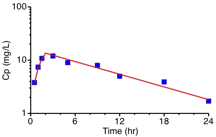
Figure 25.3.2 Semi-log Plot of Cp versus time after a 2 hour IV Infusion
From the route of administration the modeler can include details in the model that describe the administration. This might be single or multiple dose regimens. Drug may be given by IV bolus injection, IV infusion, or an extravascular route such as oral, topical or inhalation. The extravascular routes may include multiple steps such dissolution and absorption in the case of oral administration or diffusion from a patch and through the skin in the case of a topical dose. The structure of this part of the model may be derived from an understanding of the dosage form and prior knowledge however certain parameter values may need to be determined by nonlinear regression. Dissolution rate constants, multiple absorption rate constants, lag times and extent of absorption may be among the parameters to be estimated.
Consideration of the data plotted on linear and semi-log graph paper will provide more information about a suitable model. Distribution may be described with more than one compartment. More data types, such drug excreted in urine or metabolite concentrations, provide information useful in extending the model to better describe drug metabolism or excretion.
With some nonlinear programs it is possible to draw a sketch of a proposed models or select a pre-drawn model from a library (WinNonlin). Users of other programs such as Boomer may wish to draw this visualization by hand. Having a clear idea of what the model 'looks' like can be very useful in correctly defining the model with any nonlinear regression program.
Selection from a library Some programs have a collection of predefined models within a library. The user simply selects the appropriate model from this library. WinNonlin is an example of this approach. It is probably the easiest for the user IF their model is in the library. JGuiB provides a GUI which allows the user to select a model for use with Boomer.
Selection of Model Parameters Programs like Boomer provide the user with a collection of parameters, rate constants, volumes, components (compartments) and many more to provide a toolbox from which the user can build their model. This provides the user with considerable flexibility without the need to derive the equations required for the model. If the parameter toolbox contains all the required parts this can be very convenient.
Describe the Model using Computer Code For maximum flexibility the modeler can describe their model using a computer language. WinNonlin provides this flexibility with the Phoenix Modeling Language (PML). Although this approach is flexible it does also require more coding experience from the modeler.
 METHOD OF ANALYSIS

 0) Normal fitting
 1) Bayesian
 2) Simulation only
 3) Iterative Reweighted Least Squares
 4) Simulation with random error
 5) Grid Search
Non-linear regression analysis with a good number of data from one subject can be analyzed as a 'Normal Fitting'. A good number of data might be defined as twice the number of parameters to be estimated. The sampling site and sample timing should also be considered in designing the experiment.
MODEL Definition and Parameter Entry * Allowed Parameter Types * -5) read model -3) display choices -2) display parameters 0) Time interrupt 1) Dose/initial amount 2) First order rate 3) Zero order 4-5) Vm and Km of Michaelis-Menten 6) Added constant 7) Kappa-Reciprocal volume 8-10) C = a * EXP(-b * (X-c)) 11-13) Emax (Hill) Eq with Ec(50%) & S term 14) Second order rate 15-17) Physiological Model Parameters (Q, V, and R) 18) Apparent volume of distribution 19) Dummy parameter for double dependence 20-22) C = a * SIN(2 * pi * (X - c)/b) Special Functions for First-order Rate Constants 23-24) k = a * X + b 25-27) k = a * EXP(-b * (X - c)) 28-30) k = a * SIN(2 * pi * (X - c)/b) 31,32-33) dAt/dt = - k * V * Cf (Saturable Protein Binding) 34-36) k * (1 - Imax * C/(IC(50%) + C)) Inhibition 0 or 1st order 37-39) k * (1 + Smax * C/(SC(50%) + C)) Stimulation 0 or 1st order 40) Uniform [-1 to 1] and 41) Normal [-3 to 3] Probability 42) Switch parameter 43) Clone component 44-47) Four parameter logistic model 48-51) Four parameter Weibull model |
Figure 25.3.3 Parameter types available with Boomer (v3.4.7 Mar 2022)
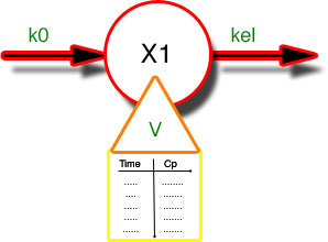
Figure 25.3.4 Diagram Illustrating a One Compartment Model with an IV Infusion
Model and Parameter Definition # Name Value Type From To Dep Start Stop 1) kel = 0.9139E-01 2 1 0 0 0 0 2) V = 13.47 18 1 1 0 0 0 3) Duration = 2.000 0 0 0 0 0 0 4) k0 = 100.0 3 0 1 0 0 1 |
Figure 25.3.5 The Model Included in the Boomer Output
Weighting function entry for [Drug] 0) Equal weights 1) Weight by 1/Cp(i) 2) Weight by 1/Cp(i)^2 3) Weight by 1/a*Cp(i)^b 4) Weight by 1/(a + b*Cp(i)^c) 5) Weight by 1/((a+b*Cp(i)^c)*d^(tn-ti)) |
Figure 25.3.6 Choices of Weight Equation provided in Boomer
More detail regarding these weight equations can be found in the Boomer manual or online.
(Section 1)
 ** FINAL OUTPUT FROM Boomer (v3.1.5) **      25 July 2005 --- 10:52:41 am

 Title:  Fit to data before and after termination of an IV infusion
 Input: From Fig2202.BAT
 Output:  To Fig2202.OUT
 Data for [Drug]          came from keyboard (or ?.BAT)
 Fitting algorithm: DAMPING-GAUSS/SIMPLEX
 Weighting for [Drug]          by 1/Cp(Obs )^2
 Numerical integration method: 2) Fehlberg RKF45
          with  1 de(s)
 With relative error   0.1000E-03
 With absolute error   0.1000E-03
 DT =   0.1000E-02     PC =   0.1000E-04 Loops =     1
 Damping =     1

(Section 2)
                    ** FINAL PARAMETER VALUES ***

  #  Name                  Value       S.D.       C.V. %  Lower <-Limit-> Upper

  1) kel                   0.91394E-01  0.431E-02   4.7       0.0       1.0
  2) V                      13.473      0.618       4.6       1.0      0.10E+03

 Final WSS =   0.886379E-01 R^2 =   0.9671     Corr. Coeff =   0.9834
 AIC =   -17.8088     Log likelihood =   8.02     Schwartz Criteria =   -17.4143
 R and R^2 - jp1     0.9856        0.9714
 R and R^2 - jp2     0.9856        0.9714

(Section 3)
 Model and Parameter Definition

  #  Name                    Value       Type From To     Dep  Start Stop

  1) kel                 =  0.9139E-01    2    1    0       0    0    0
  2) V                   =   13.47       18    1    1       0    0    0
  3) Duration            =   2.000        0    0    0       0    0    0
  4) k0                  =   100.0        3    0    1       0    0    1

(Section 4)
 Data for [Drug]          :-

 DATA #   Time       Observed      Calculated    (Weight)  Weighted residual

     1    0.000       0.00000       0.00000       0.00000       0.00000
     2   0.5000       3.80000       3.62770      0.263158      0.453408E-01
     3    1.000       7.40000       7.09336      0.135135      0.414372E-01
     4    1.500       10.8000       10.4042      0.925926E-01  0.366464E-01
     5    2.000       0.00000       13.5672       0.00000       0.00000
     6    3.000       12.0000       12.3822      0.833333E-01 -0.318495E-01
     7    5.000       9.00000       10.3137      0.111111     -0.145965
     8    9.000       8.00000       7.15558      0.125000      0.105553
     9    12.00       5.00000       5.43962      0.200000     -0.879240E-01
    10    18.00       3.90000       3.14352      0.256410      0.193969
    11    24.00       1.70000       1.81662      0.588235     -0.686003E-01

     WSS for data set  1 =   0.8864E-01
               R^2 =   0.9671     Corr. Coeff. =   0.9834
 R and R^2 - jp1     0.9856        0.9714
 R and R^2 - jp2     0.9856        0.9714

 Maximum value for [Drug]          is      12.000     at       3.000

(Section 5)
 Calculation of AUC and AUMC based on trapezoidal rule

 AUC and AUMC for [Drug]          using Observed data

       Time         Concentration      AUC             AUMC

      0.00000    (     0.00000    )
     0.500000          3.80000        0.950000        0.475000
      1.00000          7.40000         3.75000         2.80000
      1.50000          10.8000         8.30000         8.70000
      2.00000          0.00000         11.0000         12.7500
      3.00000          12.0000         17.0000         30.7500
      5.00000          9.00000         38.0000         111.750
      9.00000          8.00000         72.0000         345.750
      12.0000          5.00000         91.5000         543.750
      18.0000          3.90000         118.200         934.350
      24.0000          1.70000         135.000         1267.35
                                       153.601         1917.29

 Secondary Parameters

MRT =      12.482

 Half-life values for each first order rate constant

   Parameter   1 has a half-life of kel is       7.58

 Dose/AUC (= Clearance/F)

   Parameter   4 gives k0/AUC (CL/F) of     -0.651
|
Figure 25.3.7 Tabular and Statistical Output provided by Boomer
(Section 1) Preliminary output describing the input/output details, the fitting (optimization) algorithm, integration method and weighting scheme.
(Section 2) Best-fit parameter values with statistical information are provided. The parameter CV values, the WSS, AIC and other values provide information about the model and how well the data have been fit to the model.
(Section 3) The model definition section provides the apportunity to confirm that the model has been described correctly.
(Section 4) The data are provided next as observed x and y values, calculated y values and weight and residual information. The observed data in this table should be checked against the correct values. Systematic differences between observed and calculated values may be detected in this section if the data analysis is incorrect.
(Section 5) The program can calculate the AUC and a number of 'secondary' parameters including MRT, half-life, and Dose/AUC. A zero time point (with zero weight) must be entered for accurate estimates of AUC.
(Section 1)
Plots of observed (*) and calculated values (+)
           versus time for [Drug]         . Superimposed points (X)

    13.57      Linear                      13.57      Semi-log
 |                                       |   +
 |   +                                   |
 |                                       |    X
 |    +                                  |
 |    *                                  |  X    +
 |                                       |
 |                                       |       *
 |  X                                    |
 |       +                               |             *
 |                                       | *
 |                                       | +           +
 |       *                               |
 |                                       |
 |             *                         |
 | *                                     |                  +
 | +           +                         |                  *
 |                                       |
 |                                       |
 |                  +                    |
 |                  *                    |*                          *
 |                                       |+
 |                                       |
 |X                          *           |                           +
 |                                       |
 |                           +           |
 |                                       |
 |                                    +  |
 |                                    *  |
 |                                       |
 |                                       |
 |X  *                                   |                                    X
 |_____________________________________  |X__*_________________________________
    0.000                                  1.700
 0              <-->             24.     0              <-->             24.

(Section 2)
 Plot of Std Wtd Residuals (X)            Plot of Std Wtd  Residuals (X)
   versus time for [Drug]                   versus log(calc Cp(i)) for [Drug]

    1.955                                  1.955
 |                           X           |         X
 |                                       |
 |                                       |
 |                                       |
 |                                       |
 |             X                         |                        X
 |                                       |
 |X                                      |            X
 | XX                                    |                        X      X
 |                                       |
 0X==X=================================  0====================================X
 |    X                                  |                                  X
 |                                       |
 |                                    X  |X
 |                  X                    |                   X
 |                                       |
 |       X                               |                               X
 |                                       |
   -1.471                                 -1.471
      0.0       <-->             24.          1.8       <-->             14.
|
Figure 25.3.8 Graphical Output provided by Boomer
(Section 1) A linear and semi-log dot printer-type plot of the observed and calculated y-values versus the x-values. Systematic deviations, indicating a poor weighting scheme or model selection, may be apparent from these graphs.
(Section 2) Standardized weighted residuals versus x-value or log(calculated y value) are very useful tools for detecting a poor model or weighting scheme selection. Any obvious pattern in these plots should be explored as potential evidence of a poor fit to the data.
The Boomer control file used in this analysis is provided here and the complete output file is provided here.
The first step is to create a new project.
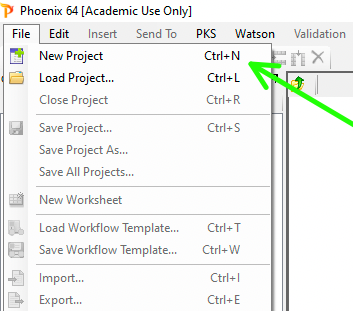
Figure 25.3.9 Creating a New Project
Next a new worksheet for the data.

Figure 25.3.10 Create a New Project
Set up two columns for Time and Concentration with units and enter the data.
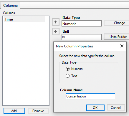
Figure 25.3.11 Columns for Time and Concentration |
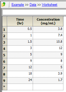
Figure 25.3.12 Columns for Time and Concentration |
We can have a look at the data first as a linear and semi-log plot to see what model might be appropriate.
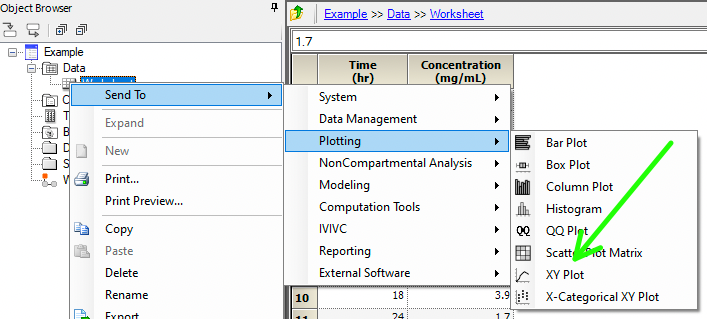
Figure 25.3.13 Send Data to XY Plot
Map Time to X and Concentration to Y and execute the plot.
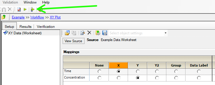
Figure 25.3.14 Map time and concentration
Starting with a linear plot, double-click on the y-axis, set it to logarithmic and we have a semi-log plot
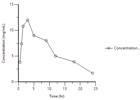
Figure 25.3.15 Linear Plot of Time and Concentration |
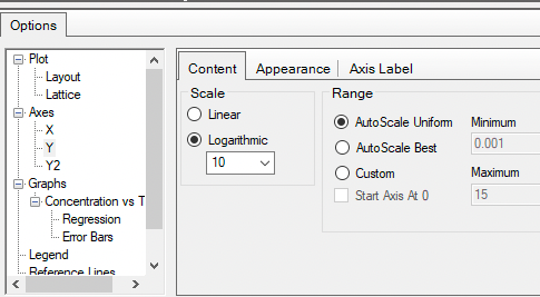
Figure 25.3.16 Set Y Axis to Logarithmic |
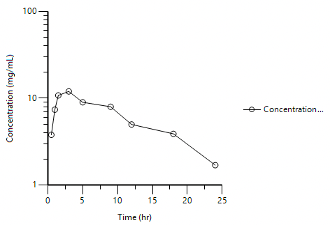
Figure 25.3.17 Semi-log Plot of Time versus Concentration |
After looking at the semi-log plot we might plan on starting with a one compartment model. We can send the Data Worksheet to a Maximum Likelihood Model.
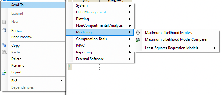
Figure 25.3.18 Create a Model for the Data
Uncheck Population as this is single subject data. Use Micro Parameterization although we could choose Clearance. Dosing by Intravenous and One compartment model. Check Infusion and Duration. For most data a Multiplicative Error model works well. This is similar to weighting by the reciprocal of the concentration squared as was done with the Boomer example. Here extended least squares is used and an initial value of 0.1 (or 10%) is entered for the fractional standard deviation.
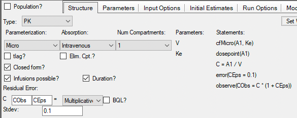
Figure 25.3.19 Set up the PK Model
We can now enter the dosing information. Two hundred milligram given over two hours starting at time zero.
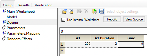
Figure 25.3.20 Enter Infusion Dose Information
Initial parameter values can be entered and confirmed and/or adjusted.
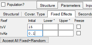
Figure 25.3.21 Enter Initial Estimate Values |
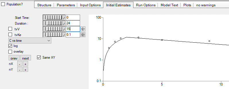 Figure 25.3.22 Confirm and/or Adjust the Initial Estimates |
Here we selected the model from a library within WinNonlin but we could build the model with a graphical or PML code. The same model can be represented by each of these methods.
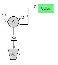
Figure 25.3.23a The Model Defined Graphically |
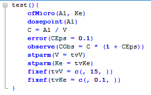
Figure 25.3.24a The Model Described with PML Code |
The columns have been mapped as before and it is time for the program to fit the data with the model by adjusting the parameter values.
Below is another example of a graphical and PML code description for a two compartment model with two covariates, one continuous (Weight) and the other categorical (Sex).
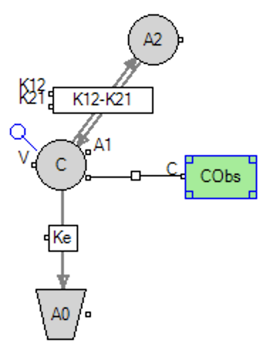
Figure 25.3.23b The Model Defined Graphically |
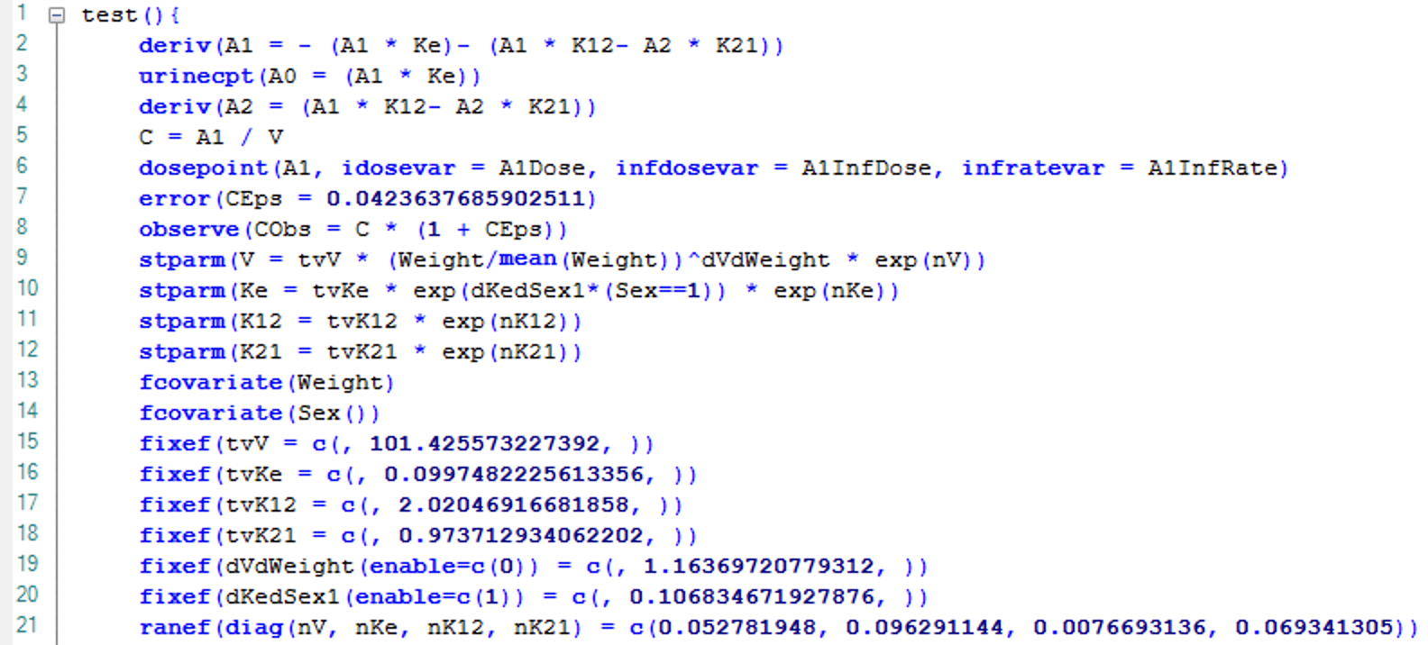
Figure 25.3.24b The Model Described with PML Code |
In Figure 25.3.24b lines 2-4 define the differential equations for the central compartment (A1), output (A0) and the peripheral compartment (A2). Amounts are converted to the observed quantity, concentration, on line 5. Line 6 describes the dosing into the central compartment. The initial error value, Eps, and the error model, here multiplicative are defined on lines 7 and 8. The adjustable parameters in the model are described on lines 9-12. Note the inclusion of Weight (on V) and Sex (on Ke) as two covariates on lines 9 and 10. On line 9 Weight has been normalized by the mean of the study observed weights. mean(Weight) could be replaced by 70 (as a fixed estimate for a population) when the study weights might not be typical. The covariates are listed in lines 13-14. Initial estimates for the adjustable parameters are included on lines 15-18. Lower and upper limits are typically not required. Lines 19-20 provide initial estimates for covariates. The last line, 21, describes initial estimates for the diagonals for the adjustable parameters.

Figure 25.3.25 Overall Statistics
The best fit values are provided along with Stder and CV%. Note that the CV% values are quite low. These are similar values to those provided by Boomer.
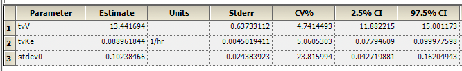
Figure 25.3.25 Best fit Parameter Values
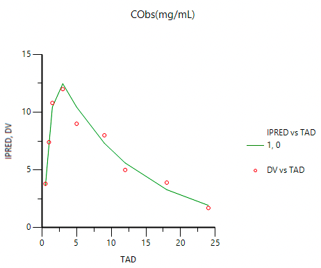
Figure 25.3.26 Linear Plot of Concentrations versus Time |
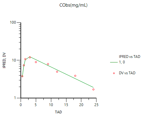
Figure 25.3.27 Semi-Log Plot of Concentrations versus Time |
Another diagnostic plot that is important to consider is the weighted residual plot. This plot can help confirm not only the selected model but also the weighting scheme.
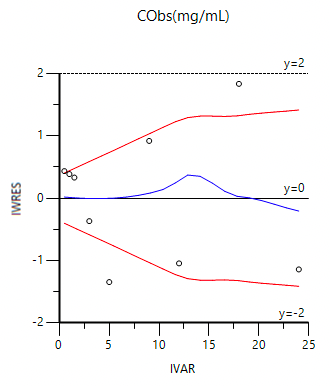
Figure 25.3.28 Weighted Residual (IWRES) Plot vesus Time (IVAR)
Material on this website should be used for Educational or Self-Study Purposes Only
Copyright © 2001 - 2026 David W. A. Bourne (david@boomer.org)
 | A game to aid in interpreting Prescription Sig instructions See how many Sigs you can catch before you run out of lives |
|