Integrating Differential Equations using Laplace Tranforms
return to the Course index
previous | next
Laplace transforms are a convenient method of converting differential equations into integrated equations, that is, integrating the differential equation. It is similar to the use of logarithms to multiple or divide numbers. To multiple two numbers we convert each number into their respective logarithm and add. The sum is converted into the 'anti'-logarithm and the product of the original numbers is the result. For division, the logarithm of the two numbers are subtracted before obtaining the answer by taking the anti-logarithm.
Differential equations can be converted into the integrated form using Laplace transforms by following a number of straight forward steps.
- Write the differential equation. Using the approach presented on the previous page you need to write the differential equation for the system of interest.
- Take the Laplace transform of each differential equation using a few transforms. We transform the equation from the t domain into the s domain. For most pharmacokinetic problems we only need the Laplace transform for a constant, a variable and a differential.
- Use some algebra to solve for the Laplace of the system component of interest. Often the Laplace of a component 'up-stream' will need to be solved first and substituted into the equation of interest.
- Finally the 'anti'-Laplace for the component is determined from tables such as that below or by using the 'finger-print' method describe later.
In step two above, only three Laplace transforms are necessary for most of the linear of pharmacokinetic systems that you might encounter. These are:
The Laplace of a constant:

The Laplace of a variable (i.e. amount in a component of the model; e.g. X1):

The Laplace of the differential of a variable (e.g. dX1/dt):

Time for some examples
IV Bolus - Linear one compartment model
The IV bolus does is placed in component one at zero time. Elimination is by a single first order process described by the rate constant kel (elimination rate constant). The scheme can be describe by Figure 2.8.1

Figure 2.8.1 Linear one compartment model with one elimination process
- Write the differential equation for X1. There is only one component.
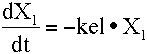
- Transform the equation into the Laplace form
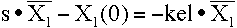
- Rearranging and solving for L(X1). Substitute Dose for X1(0).
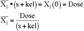
-
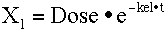
The final result can be determined from the Laplace Transform table (below - line 3 with A == Dose: a == kel).
Additional problems and answers are available.
References
return to the Course index
This page was last modified: Sunday, 28th Jul 2024 at 4:41 pm
Privacy Statement - 25 May 2018
Material on this website should be used for Educational or Self-Study Purposes Only
Copyright © 2001 - 2026 David W. A. Bourne (david@boomer.org)
 | Pharmacy Math Part One
A selection of Pharmacy Math Problems |
 |