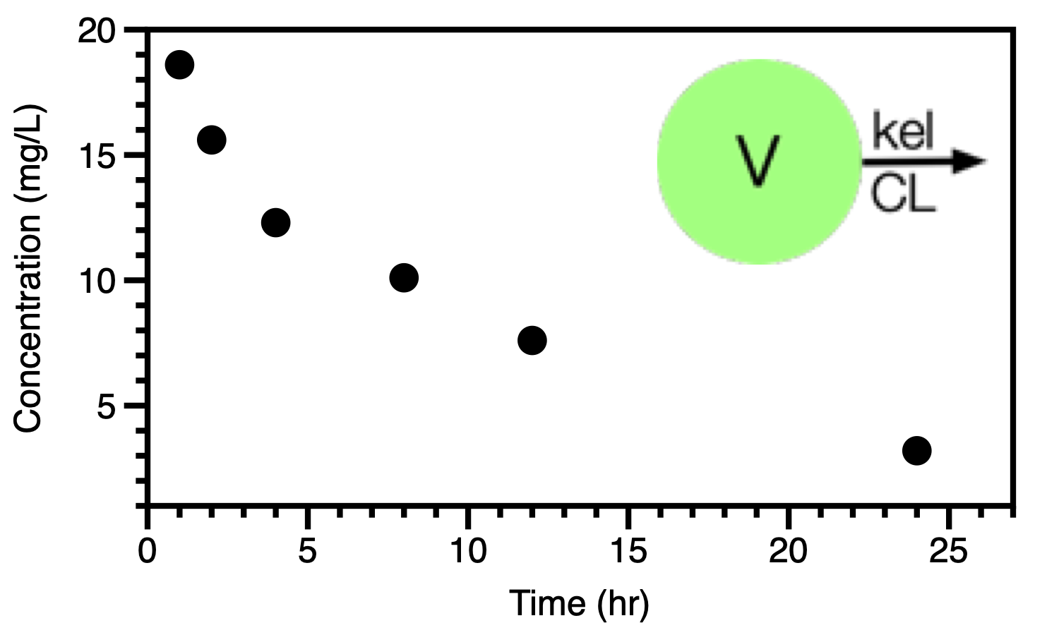
Figure 25.2.1 Linear plot of concentration versus time data (Subject 1)
return to the Course index
previous | next
During the development of new drugs and new dosage forms numerous pharmacokinetic studies in animals (pre-clinical) and humans (clinical) are performed. These and other studies will produce large amounts of data. Even a simple six subject study will provide considerable data. A full page of data.
| Time (hr) | Concentration (mg/L) |
Time (hr) | Concentration (mg/L) |
Time (hr) | Concentration (mg/L) |
|---|---|---|---|---|---|
| 1.0 | 18.6 | 1.0 | 19.3 | 1.0 | 19.3 |
| 2.0 | 15.6 | 2.0 | 15.8 | 2.0 | 14.5 |
| 4.0 | 12.3 | 4.0 | 11.5 | 4.0 | 12.5 |
| 8.0 | 10.1 | 8.0 | 9.8 | 8.0 | 10.3 |
| 12.0 | 7.6 | 12.0 | 6.5 | 12.0 | 6.9 |
| 24.0 | 3.2 | 24.0 | 2.1 | 24.0 | 3.5 |
| Subj #1 Wt 76 Kg Dose 200 mg | Subj #2 Wt 74 Kg Dose 200 mg | Subj #3 Wt 54 Kg Dose 150 mg | |||
| Time (hr) | Concentration (mg/L) |
Time (hr) | Concentration (mg/L) |
Time (hr) | Concentration (mg/L) |
| 1.0 | 18.9 | 1.0 | 19.5 | 1.0 | 18.7 |
| 2.0 | 14.6 | 2.0 | 14.7 | 2.0 | 14.9 |
| 4.0 | 12.7 | 4.0 | 12.3 | 4.0 | 12.3 |
| 8.0 | 10.3 | 8.0 | 10.7 | 8.0 | 10.3 |
| 12.0 | 7.5 | 12.0 | 6.9 | 12.0 | 7.9 |
| 24.0 | 3.3 | 24.0 | 4.1 | 24.0 | 3.5 |
| Subj #4 Wt 58 Kg Dose 150 mg | Subj #5 Wt 94 Kg Dose 250 mg | Subj #6 Wt 82 Kg Dose 225 mg | |||
and numerous plots of the data.
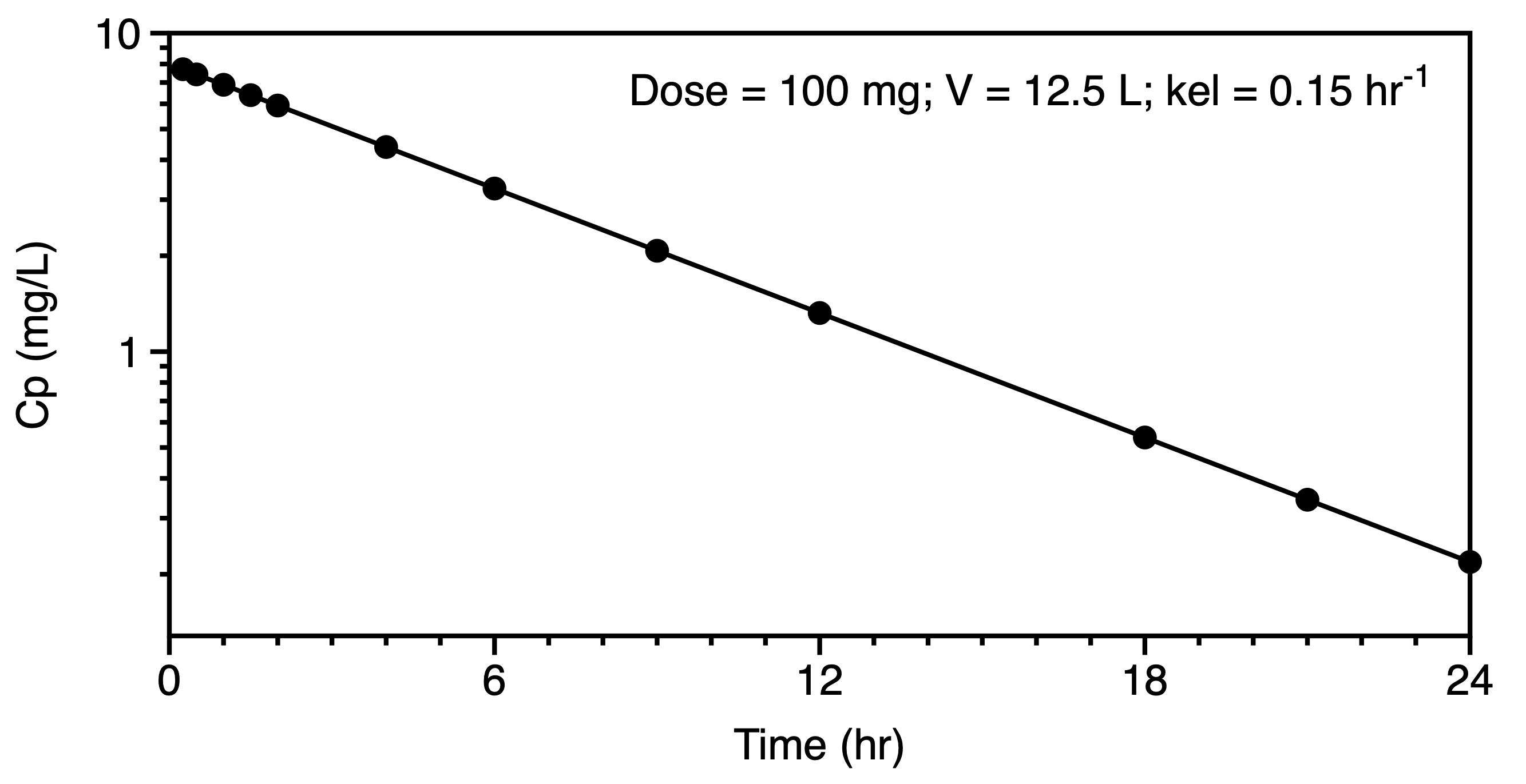
Figure 25.2.1 Linear plot of concentration versus time data (Subject 1)
Figure 25.2.1 illustrates one of these plots of the data from just one subject. Also portrayed in Figure 25.2.1 is a simple one compartment model with two parameters, V and kel or CL. We can start the data analysis with a semi-log plot of the data in Table 25.2.1.
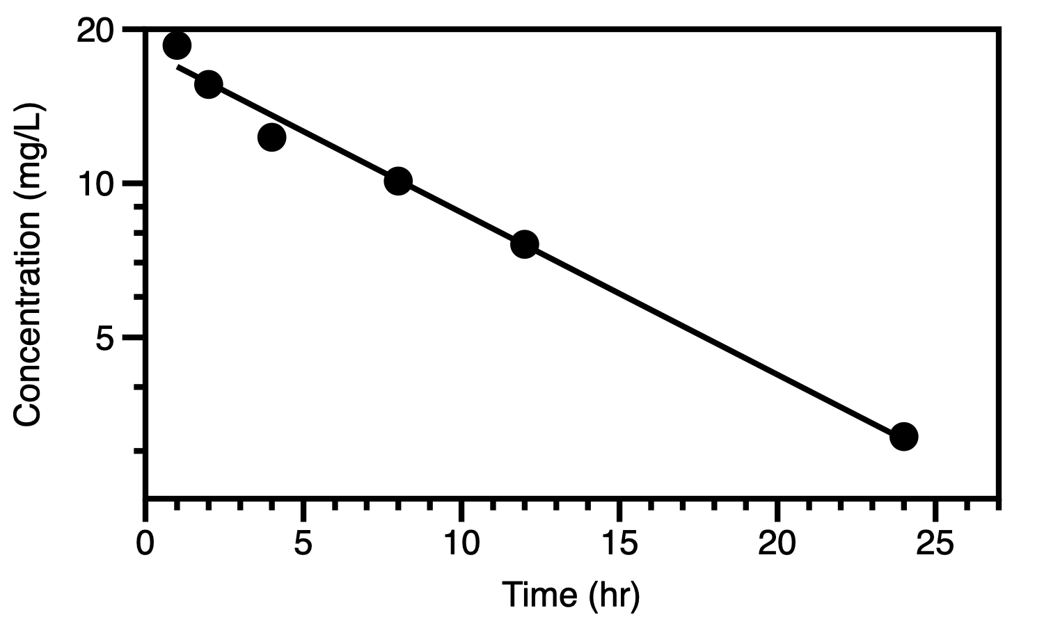
Figure 25.2.2 Semi-log plot of concentration versus time data (Subject 1)
Values for V and kel can be determined from the intercept and slope of the best-fit line.
If we model all the data in Table 6.2.1 we can summarize all these data with the model and averaged parameter values.
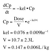
Table 25.2.2 Simple model and parameter values
Thus the data from six subjects can be summarized with an equation (model) and parameter values for the model.
When we quantitate observations and model data we can better understand what is happening in the system under study. Correlation can be explored between the parameter values and other observations that may be collected. Table 6.3.1 provides pharmacokinetic parameters from a number of subject as well as some of the data that might be collected from a patient's hospital chart.
| Subject | Weight | Sex | CLCr | Dose | kel | V |
|---|---|---|---|---|---|---|
| 1 | 75 | F | 102 | 200 | 0.38 | 15.2 |
| 2 | 68 | F | 34 | 175 | 0.13 | 13.2 |
| 3 | 65 | F | 21 | 175 | 0.10 | 13.1 |
| 4 | 98 | M | 54 | 250 | 0.28 | 19.4 |
| 5 | 56 | M | 65 | 150 | 0.32 | 11.2 |
| 6 | 76 | M | 76 | 200 | 0.36 | 15.5 |
| ... | ... | ... | ... | ... | ... | ... |
| ... | ... | ... | ... | ... | ... | ... |
With these data we could explore some of these correlations. For example plotting the kel measured in these patient versus the clinical parameter creatinine clearance may result in a plot such as Figure 25.2.3.
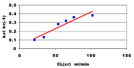
Figure 25.2.3 Linear plot of observed kel versus creatinine clearance
Figure 25.2.3 suggests that there is a significant correlation between elimination of this drug and renal function as expressed by the creatinine clearance. A large fraction of the drug dose must be excreted into urine. If renal function is poor elimination would be impaired and the drug dosage regimen should be adjusted appropriately. We could also explore the relationship between apparent volume of distribution and creatinine clearance.
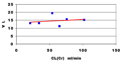
Figure 25.2.4 Linear plot of apparent volume of distribution and creatinine clearance
In Figure 25.2.4 we see that there is little correlation between the apparent volume of distribution and creatinine clearance.
In another study we might look at the effect of drug dose and pharmacokinetic parameters. Some data are shown in Table 25.2.4.
| Dose 25 mg | Dose 100 mg | Dose 500 mg | |||
| Time (hr) | Concentration (mg/L) |
Time (hr) | Concentration (mg/L) |
Time (hr) | Concentration (mg/L) |
|---|---|---|---|---|---|
| 0.0 | 2.03 | 0.0 | 8.13 | 0.0 | 40.6 |
| 0.5 | 1.83 | 0.5 | 7.62 | 0.5 | 39.8 |
| 1.0 | 1.65 | 1.0 | 7.14 | 1.0 | 38.9 |
| 2.0 | 1.34 | 2.0 | 6.22 | 2.0 | 37.2 |
| 3.0 | 1.07 | 3.0 | 5.38 | 3.0 | 35.6 |
| 4.0 | 0.86 | 4.0 | 4.61 | 4.0 | 33.9 |
| 6.0 | 0.54 | 6.0 | 3.29 | 6.0 | 30.7 |
| 9.0 | 0.26 | 9.0 | 1.85 | 9.0 | 25.9 |
| 12.0 | 0.12 | 12.0 | 0.97 | 12.0 | 21.4 |
| 18.0 | 0.02 | 18.0 | 0.23 | 18.0 | 13.2 |
| 24.0 | 0.01 | 24.0 | 0.05 | 24.0 | 6.6 |
Plotting these data on semi-log graph paper provides three lines with different slope and shape.
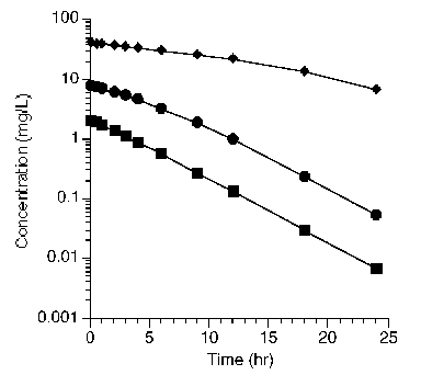
Figure 25.2.5 Semi-log plot of concentration versus time after three different doses
It would appear that these data represent nonlinear or saturable pharmacokinetics (which was discussed in more detail in Chapter 21). A model which could explain these data are shown in Figure 25.2.6 along with a plot of AUC versus dose. This is another representation of these and more data collected after additional dose values which illustrates the nonlinear model.
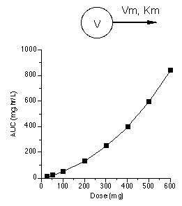
Figure 25.2.6 Linear plot of AUC achieved after various doses
These and other mechanisms can be explored by modeling pharmacokinetic data.
Once we have a model and parameter values we can use this information to make predictions. For example we can determine the dose required to achieve a certain drug concentration.
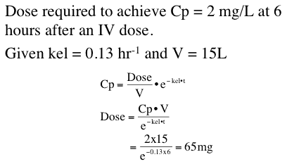
Figure 25.2.7 Dose required to achieve a certain plasma concentration
Using these data we can calculate (or predict) the drug concentrations at various time up to and including the six hours requested.
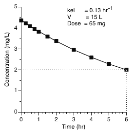
Figure 25.2.8 Plasma concentration versus time after a 65 mg IV bolus dose
We can also predict drug concentrations after a specified drug dosage regimen.
Figure 25.2.9 Concentrations after multiple IV Bolus doses
With this information we can predict drug plasma concentrations after multiple 100 mg IV bolus doses every 12 hours.
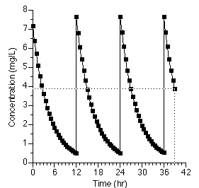
Figure 25.2.10 Linear plot of drug concentration versus time after multiple IV Bolus doses
With more extensive models even more involved predictions or calculations can be performed.
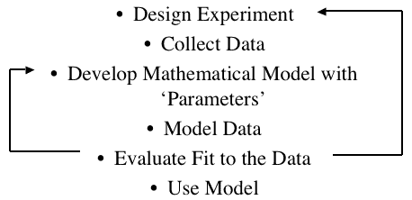
Figure 25.2.11 A general approach to modeling
As mentioned earlier, pharmacokinetic models are described as equations or formulas. in general there is a dependent variable (y variable) expressed as a function of independent variable(s) (x variable) with various constants and/or parameters.

Figure 25.2.12 The dependent variable is a function of the independent variable(s) and ...
Constants and parameters may be interchangeable or considered very similar. From a modeling point of view parameters are values that are determined by the computer program. Constants are terms that are held fixed during the modeling process.
Mathematical models take many forms. The simplest form is probably the equation for a straight line.
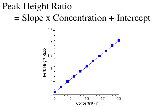
Figure 25.2.13 Linear plot of y versus x for a straight line
In Figure 25.2.13 peak height ratio is the dependent variable and concentration is the independent variable. Slope and intercept are parameters. This is an equation that is very useful for standard curves used in drug analysis.
A pharmacokinetic model is the next example. This is a very simple example which is a not a straight line unless it is transformed. As an exponential equation there was usually two parameters, kel and V, with dose as the constant.
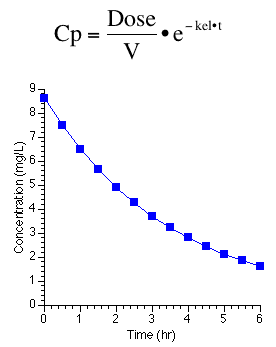
Figure 25.2.14 Linear plot of drug concentration versus time
A third example is a pharmacological equation relating drug effect to drug concentration using a form of the Hill equation. The parameters in this model are EMax, EC50% and γ. We'll see more of this type of model in the next chapter.
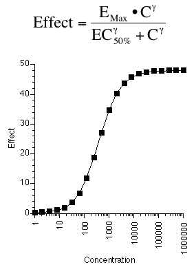
Figure 25.2.15 Linear plot of drug effect versus drug concentration
The first step towards successfully modeling pharmacokinetic data is to consider the route of administration and the data available. Data collected after an intravenous (IV) bolus may be the easiest to analyze as there are no absorptions steps to consider. The bolus dose should be well defined and it should not be necessary to estimates its value. An IV infusion adds an administration step, a rate of infusion and possibly a duration if the infusion is stopped. Again, both of these parameters should be well know. A dose given by mouth or as a intramuscular (IM) injection require the addition of an administration step. This might be a simple one compartment process or it could be more complex. Solubility, stability and site of absorption can add to the complexity of the absorption step and the overall model. Samples other than blood or plasma may be available. Unchanged drug and metabolite in urine samples can add another dimension to the model selection process. The absorption, distribution, metabolism and excretion (ADME) processes may not be all first order. Data collected after different doses can be useful, as seen in the figure below.

|

|
Data collected after multiple dosing also adds the model detail. At this point we could envisage potential models with rapid distribution and a single compartment representing the body.
We might now move to the consideration of data plotted on linear and semi-log graphs. These graphs should confirm our thought regarding the administration and elimination, metabolism and excretion, of the drug and metabolite. A distribution phase may suggest a multi compartment pharmackinetic model. Even after extravascular administration such as oral dosing a distribution phase may be evident in the semi-log plot. Compare the plots in Figures 6.6.6 and 6.6.7. The early data in the second semi-log plot indicate a deviation from the terminal straight line at early time points, leading one to consider a two or three compartment distribution as part of the model.
|
|
|
|
For a simple one compartment model after an IV bolus the equation for concentration versus time can be expressed in logarithmic form as a straight line as illustrated by the right hand plot in Figure 6.6.6. The slope and intercept can provide estimates of V and kel. Estimating the area under the concentration versus time curve (AUC) can provide an estimate of clearance. Initial estimates for the parameters of a two compartment model can be determined by the method of residual (aka: curve striping or feathering the curve). In a similar fashion the absorption and elimination rates constant for oral administration, one compartment model can be estimated using the method of residuals.
Another approach that can be quite useful is to perform a non compartmental analysis (NCA) of the data and derived estimates in the process.
Some computer software can use a range of typical parameter values and preform a multi-dimensional grid search to find a region near the minimum sum of the weighted residuals.
Least squares criteria refers to the formula used as a measure of how well the computer generated line fits the data. Thus it is a measure of the total of the differences between the observed data and the calculated data point. Most commonly with pharmacokinetic modeling these differences are measured in the vertical direction. That is, in the y axis values. Usually time is the x or independent variable and it should be possible to measure time accurately. The y axis or dependent variable, usually concentration, often involves an assay method which means there may be error (or variation) in each result.
Figure 25.2.18 Linear plot of Cp versus time illustrating error between observed data and calculated line
Again, usually the residual or error is assumed to be in the vertical direction although there are programs available that are capable of looking at oblique error in both the x and y direction. For the rest of our modeling discussion we will assume that the error is in the y axis variable only.
Looking at an individual data point and the calculated value with the same x value the residual can be expressed as a simple subtraction.
Equation 25.2.1 Residual in the y direction
The problem is that over all the data points there might be high positive and high negative residuals that might cancel out. An absolute difference would solve this problem but squaring the residual is better statistically and achieves the same result.
Equation 25.2.2 Residual in the y direction squared
This gives us an equation of the residual for one data points. To complete the calculation we need to include the residuals for all the data points. This is called the sum of the squared residuals (SS).
Equation 25.2.3 Sum of the squared residuals
Finally we need to take the error in each data point as a separate value. That is the error may be different for each measured, observed data point. We can compensate for this by applying a weight to each residual thus the usual criteria for a best fit is a minimum sum of the weighted, squared residuals (WSS).
Equation 25.2.4 Weighted sum of squared residuals
The job of the computer program is to produce a minimum value for WSS. This is also called the objective function. The fit with the minimum value of the WSS or objective function represents the best fit according to the least squares criteria. Inspection of Equation 25.2.4 leads to the conclusion that this can be achieved by changing the calculated values (Ycalculated,i) by changing the parameter values. Other approaches such extended least squares, iterative reweighted least squares, Bayesian analysis and population analysis methods use modifications of this objective function.
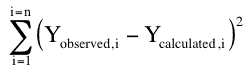
The data analysis computer program must change the parameter values to achieve a minimum value for the weighted sum of the squared residuals (WSS). This can be illustrated by changing the slope and intercept for the equation for a straight line. The calculated WSS changes with each change in the parameter values.
Figure 25.2.19 Effect on WSS of adjusting slope and intercept
Click on the figure to download an Excel® example
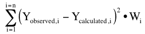
Another more involved example is the calculation of the best fit to data collected after oral administration. Two of the parameters involved in this model are ka and kel. Adjusting the values of these parameters provide different values for the WSS.
Figure 25.2.20 Effect on WSS of adjusting kel and ka
Click on the figure to download an Excel® example
Material on this website should be used for Educational or Self-Study Purposes Only
Copyright © 2001 - 2026 David W. A. Bourne (david@boomer.org)
 | A game to aid recognizing drug structures See how many structures you can name before you run out of lives |
|