Chapter 27 Numerical Integration

return to the Course index
previous | next

Runge-Kutta Method

Runge-Kutta methods are also point slope methods but were designed to provide improved accuracy with larger stepsizes and without the need to higher differentials (beyond the first derivative) of the function of interest. There are a few more calculations. There is a whole family of Runge-Kutta methods. A commonly used method (in pharmacokinetic programs) is the fourth order. There are four steps in the calculation, that is, for each 'step'.

Fourth Order Runge-Kuuta Equations

Figure 27.3.1 Equations for the Fourth Order Runge-Kutta Method

Notice the time at which the first derivatives (f terms, i.e. differential equations) are determined. Calculations are made at the initial time, two at half the stepsize beyond the initial time and at the final time. These four calculations allow the use of larger overall stepsizes with good accuracy. The method can be represented graphically.

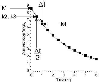
Figure showing calculation according to the Runge-Kutta method

Figure 27.3.2 Plot of Cp versus time Illustrating the 4th order Runge-Kutta Method

Compare the accuracy using the fourth order Runge-Kutta with the accuracy achieved with Euler's method. As with the previous Euler's method example the initial value is 100 and the rate constant is 0.3 hr^-1.

**Table 27.3.1 Table Illustrating Accuracy Achieved with 4th order Runge-Kutta Method**
Stepsize	Numerical	Analytical
1	74.084	74.082
0.5	86.071	86.071
0.25	92.774	92.774
0.1	97.044	97.045

This seems to be an efficient method of numerically integrating differential equations. However, what stepsize should we use? We could repeat the calculation with a smaller stepsize, say half the previous value. If the two estimates were within limits we could confirm that they were both satisfactory. The problem is that this would require 8 more calculations. That is the original four calculation plus the additional 8 for the re-calculation with the stepsize half the previous value. If the accuracy is not sufficient even more calculations would be needed. One solution to this inefficiency is the Runge-Kutta-Fehlberg method.

Runge-Kutta-Fehlberg Method (RKF45)

The Runge-Kutta-Fehlberg method (Fehlberg, 1969) takes one additional calculation per step and uses it to determine the appropriate stepsize. This makes the method very efficient for ordinary problems of numerical integration. This is the default method I would recommend for use with Boomer.

Reference

Fehlberg, E. 1969 Low-order Classical Runge-Kutta Formulas with Stepsize Control and Their Application to Some Heat Transfer Problems, NASA Technical Report, NASA TR R-315.
Runge-Kutta methods at Wikipedia
Runge-Kutta-Fehlberg methods at Wikipedia

This page was last modified: Sunday, 28th Jul 2024 at 5:08 pm

Privacy Statement - 25 May 2018

Material on this website should be used for Educational or Self-Study Purposes Only

Name the Drug
A game to aid recognizing brand versus generic drug names
See how many names you can catch before you run out of lives