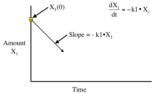
Figure 27.2.1 Linear plot of amount versus time
return to the Course index
previous | next
Figure 27.2.1 Linear plot of amount versus time
Euler's method is a point-slope method
The point (starting point) is the initial value for the each calculation.
The slope is calculated from the differential equation using the value, X1, at the next time point.
Thus, for this example of a one compartment model after an IV Bolus dose;
Point = X1(0)
and Slope = - k1 • X1(0)
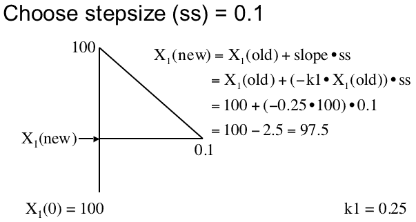
Figure 27 Calculation of the next data point
With X1(0) = 100 mg, k1 = 0.25 hr-1 and stepsize = 0.1 the new value is 97.5 mg. For comparison, the concentration using the exact equation of Dose • e-k1 • 0.1 = 100 • e-0.25 • 0.1 = 97.53. Not too bad, about 0.03% error.
We can extend the calculation out for as long as we like. The table below provides the calculation out for 0.5 hours.
| Time | ΔX1 | X1 |
|---|---|---|
| 0.0 | 100 | |
| 0.1 | -2.50 | 97.50 |
| 0.2 | -2.44 | 95.06 |
| 0.3 | -2.38 | 92.68 |
| 0.4 | -2.32 | 90.36 |
| 0.5 | -2.26 | 88.10 |
Note the exact answer is Dose • e-k1 • 0.5 = 100 • e-0.25 • 0.5 = 88.25. An error of 0.17%.
Euler's method calculations are based on the equation for the differential equation, the slope.

Figure 27.2.1 Equations used in Euler's Method Calculation
The equations above can be repeated out to what ever time is required. Remember this is a straight line approximation to a line that is curved. The method is only accurate if the step size is not too big. We can see this with another example. Using parameters Cp0 = 100 and kel = 0.3 hr-1 we can explore the effect of step size. In the table below either 1, 2, 4, or 10 steps are taken to get from time 0 to time 1.
| Stepsize | Numerical | Analytical | % Error | Number of Steps |
|---|---|---|---|---|
| 1 | 70.0 | 74.08 | 5.51 | 1 |
| 0.5 | 85.0 | 86.07 | 1.24 | 2 |
| 0.25 | 92.5 | 92.77 | 0.30 | 4 |
| 0.1 | 97.0 | 97.04 | 0.05 | 10 |
Note the error drops from over 5 % to 0.05 % by decreasing the stepsize by 10. After 10 steps the error with the smaller stepsize would be approximately 0.05 %. A 100 fold improvement for a 10 fold increase in computational cost.
The effect of the larger stepsize, in this case 1, on the calculation is illustrated below.
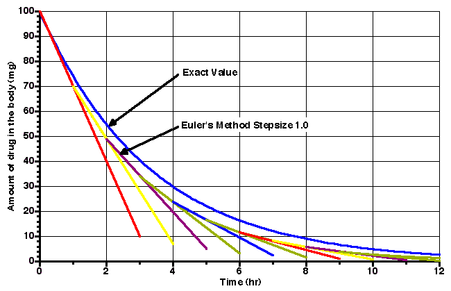
Figure 27.2.3 Plot of Amount versus Time calculated exactly and using Euler's method
Notice the divergence between the slope at each time point and the exact curve, as time progresses.
Euler's method is quite straight forward and easy to program but it requires small sizes for an accurate calculations. The smaller the stepsize the larger the number of steps and time and computational cost required to achieve a satisfactory answer. Other point-slope methods, such as the Runge-Kutta methods, tend to be more efficient, giving more accurate answers with relatively fewer steps.
Euler's method is not very efficient but it is easy to understand as a simple example of a point-slope method. For this method to be useful small steps sizes are required and an adaptive method to adjust the step size. For example, comparing results from two half-step sizes with a full step. Comparing the result after two 0.05 steps with the result after one 0.1 step, halving the steps if the error or difference is too large. Wikipedia entry for Euler's method.
Spreadsheet Example to Explore Stepsize Adjustment using Euler's Method. Numbers Excel
Material on this website should be used for Educational or Self-Study Purposes Only
Copyright © 2001 - 2026 David W. A. Bourne (david@boomer.org)
 | An iPhone app that facilitates the geotagging of Bird Count stops and the return to the same stops during the next and subsequent Bird Count sessions |
|