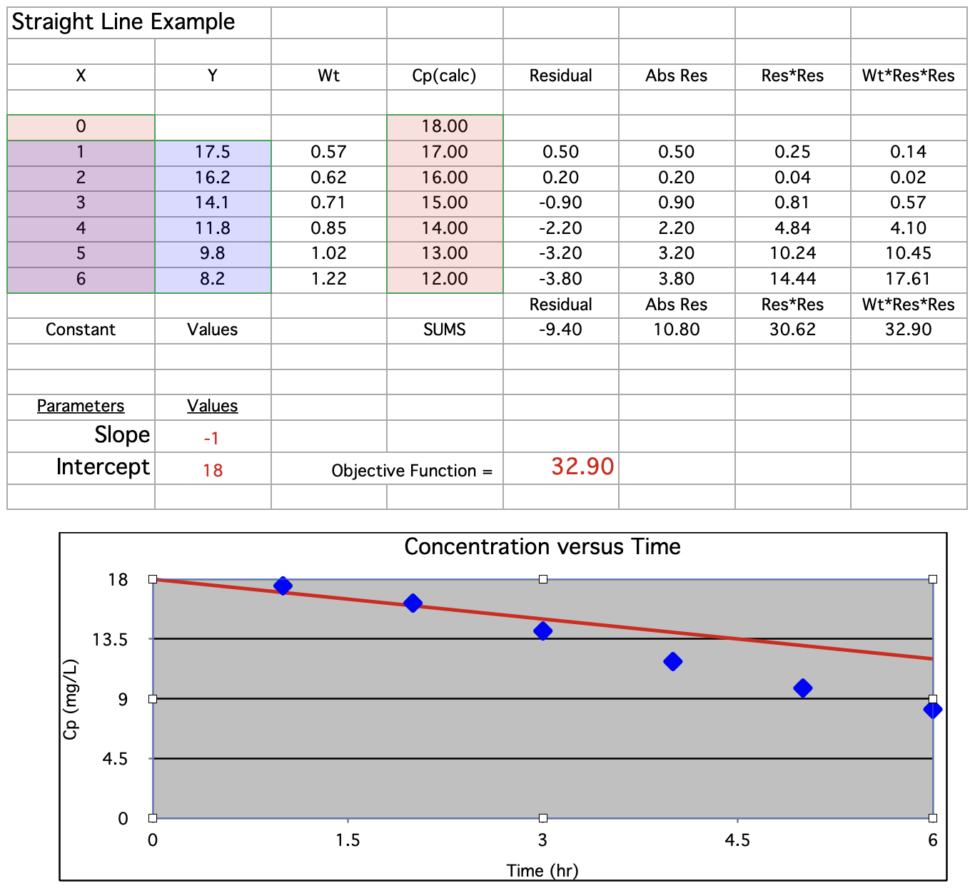
Figure 28.2.1 Numbers™ Spreadsheet Illustrating a best-fit to a straight line
return to the Course index
previous | next
Figure 28.2.1 Numbers™ Spreadsheet Illustrating a best-fit to a straight line
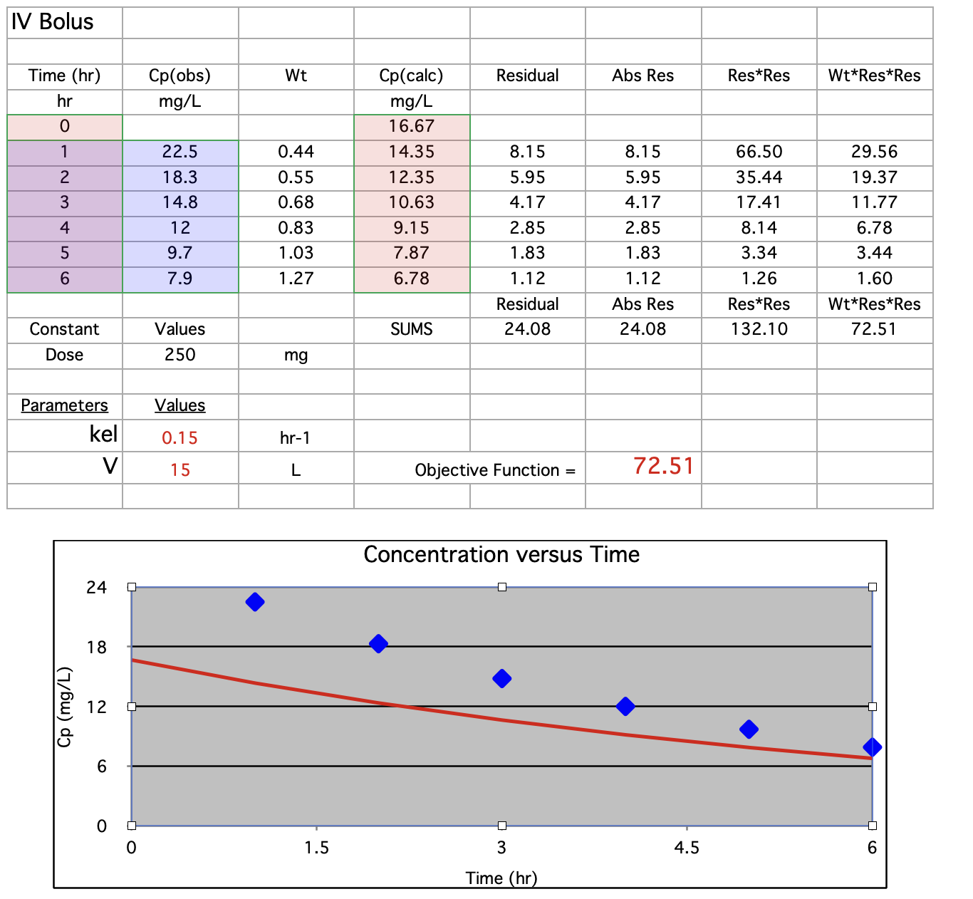
Figure 28.2.2 Numbers™ Spreadsheet Illustrating a best-fit to a one Compartment Model - IV Bolus
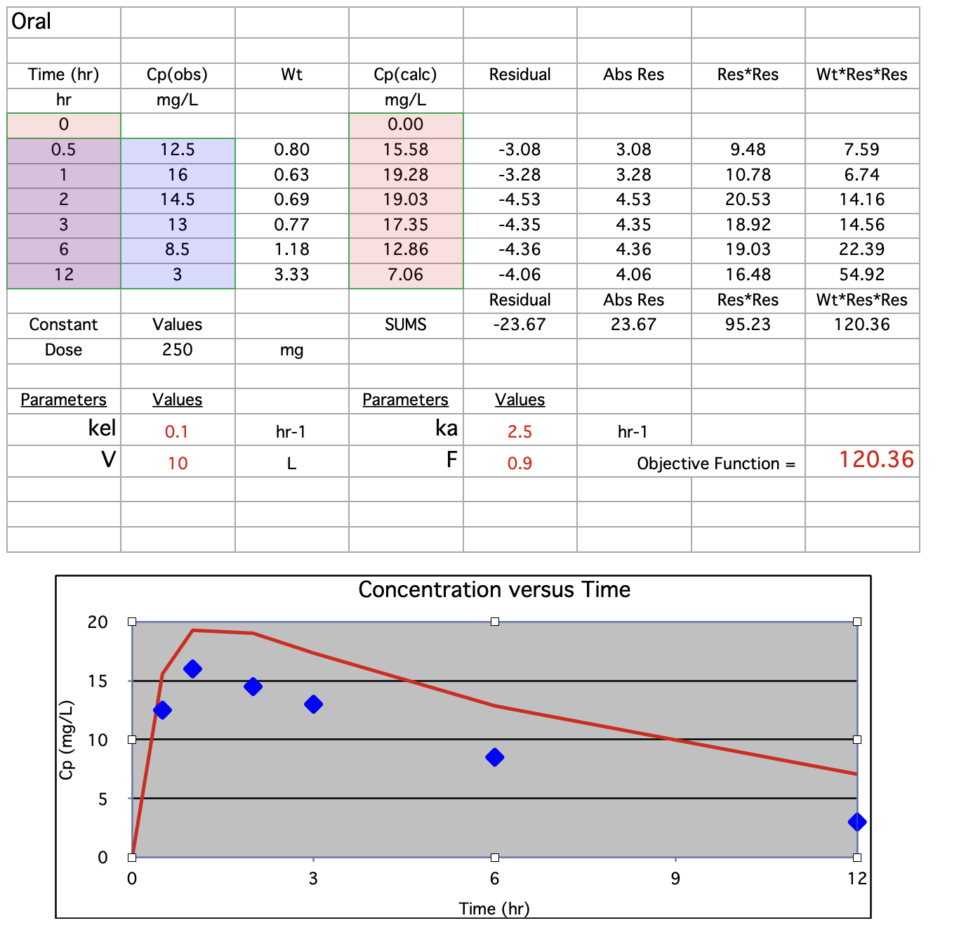
Figure 28.2.3 Numbers™ Spreadsheet Illustrating a best-fit to a one Compartment Model - Oral
You can download each of these worksheets (actually all in the same file) and try your own version of optimization. Change the parameter values and watch the value for the objective function, WSS, change. With a little 'fiddling' you should be able to get close to a best-fit. Try the straight line example first.
Download the Numbers - Spreadsheet or Excel - Spreadsheet
Note, in contrast to your adjusting the parameter values and seeing the effect the digital computer does this best-fit optimization blind-folded. Before we move onto how the digital computer does this magic lets look briefly at another type of computer.
My first computer assisted pharmacokinetic modeling at the University of Kentucky was performed with an analog computer, similar to these Electronic Associates Inc. (EAI TR-20 and TR-10) analog computers.
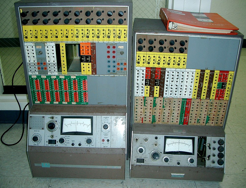
Figure 28.2.4 Patch Panel EAI TR-20 and TR-10 Analog Computers
An image by Steve Jurvetson via Wikimedia Commons.
The pharmacokinetic model was constructed by connecting components with patch cords, not shown. Adjustment of the potentiometers (top on each image) was equivalent to adjusting the rate constants of the model. Output was to an oscilloscope. Optimization was performed by 'twiddling' with the potentiometers and watching the oscilloscope for a match with the data. Great fun!
Numerical integration as the speed of light...electron.
Material on this website should be used for Educational or Self-Study Purposes Only
Copyright © 2001 - 2026 David W. A. Bourne (david@boomer.org)
 | Pharmacy Math Part Two A selection of Pharmacy Math Problems |
 |
.jpg)