Integrated equation

We can calculate the line (in Figure VIII-1) using the integrated form of the equation. Starting with the differential equation we can substitute Xg = Xg *e^{-ka * t}. The integration process won't be described here but a reference, which describes the Laplace transform method of integration [1], can be presented. This method makes integration as easy as the logarithmic transform makes multiplication and division easier.

If we use F * DOSE for Xg⁰ where F is the fraction of the dose absorbed, the integrated equation for Cp versus time is :-

Equation VIII-4

Notice that the right hand side of this equation (Equation VIII-4) is a constant multiplied by the difference of two exponential terms. A biexponential equation.

We can plot Cp as a constant times the difference between two exponential curves (see Figure II-1). If we plot each exponential separately.

Figure VIII-3, Linear Plot of e^{-ka x t} versus Time for Two Exponential Terms

Notice that the difference starts at zero, increases, and finally decreases again.

Plotting this difference by

gives Cp versus time.

Figure VIII-4, Linear Plot of Cp versus Time

We can calculate the plasma concentration at anytime if we know the values of all the parameters of Equation VIII-4.

We can also calculate the time of peak concentration using the equation:-

As an example we could calculate the peak plasma concentration given that F = 0.9, DOSE = 600 mg, ka = 1.0 hr^-1, kel = 0.15 hr^-1, and V = 30 liter.

= 2.23 hour

= 21.18 x [ 0.7157 - 0.1075] = 12.9 mg/L

As another example we could consider what would happen with ka = 0.2 hr^-1 instead of 1.0 hr^-1

= 5.75 hour

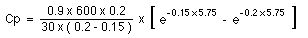
= 72 x (0.4221 - 0.3166) = 7.6 mg/L lower and slower than before

Copyright 2001 David W.A. Bourne