PHAR 4634 - Chapter 9 Page 2

Calculation of ka

Method of residuals

Starting with the equation for Cp versus time

Equation IX-1 Cp versus Time after Oral Administration

this can be written as

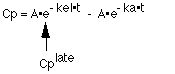
Cp = A * e^{-kel * t} - A * e^{-ka * t}

where A =

Figure IX-1, Semi-log Plot of Cp versus Time Showing a Straight Line at Longer Time

Using a JAVA aware browser you can create your own version of Figure IX-1.

Plasma Concentration versus Time Plots

If one of the rate constants (ka or kel) is much larger than the other, the method works best if the difference is at least five times, then the faster differential will approach zero more quickly, and at later times can be ignored. If we plot Cp versus time on semi-log graph paper we will see that the slope will approach a straight line.

The equation for this straight line portion can be obtained from the equation for Cp by setting the faster term (usually e^-ka*t) to zero:

Figure IX-2, Semi-log Plot of Cp versus Time Showing Cplate, Slope, and Intercept

then

Cp^late = A * e^{-kel * t}

and plotting Cp^late versus time gives a straight line on semi-log graph paper, with a slope (ln) = -kel and intercept = A.

Now

therefore

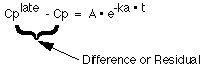
Plotting the ln (Residual) versus time should give another straight line graph with a slope (ln) equal to - ka and the same intercept as before, i.e. A

ln (Residual) = ln (A) - ka * t

Figure IX-3, Semi-log Graph of Cp versus Time Showing Residual Line

This is the method of residual or "feathering".

It can give quite accurate values of kel, ka, and V/F if :-

i) One rate constant is at least five times larger than the other

and

ii) Both absorption and elimination are first order processes.

Table IX-1: Example Data for the Method of Residuals

Time
(hr) Plasma
Concentration
(mg/L) Cp(late)
(mg/L) Residual
[Col3 - Col2]
(mg/L)

0.25 1.91 5.23 3.32

0.5 2.98 4.98 2.00

0.75 3.54 4.73 1.19

1.0 3.80 4.50 0.70

1.5 3.84 4.07 0.23

2.0 3.62 3.69 0.07

3.0 3.04

4.0 2.49 Residual

5.0 2.04 Cp^late = 5.5 * e^{2.05 * t}

6.0 1.67 = 5.5 * e^{0.2 * t}

7.0 1.37

Figure IX-4, Plot of Cp and Residual versus Time

The objective of this panel is to illustrate the Method of Residuals for determining information about the drug absorption process.

First: Draw the Cp^late line by changing the intercept (A(k1)) and slope (k1) values. Press the Cp(late) button to plot the line and calculate the residual values.

Second: Draw the Residual line by changing the intercept (A(k2)) and slope (k2) values. Press the Plot Residual button to plot the residual line.

By trial and error best fit lines can be drawn and the parameters determined.

Up to eleven (11) different data points can be entered instead of the example data provided. Leave fields empty if there are fewer than 11 data points in your data set.

This figure requires that your browser is Java capable.

For practice try calculating the absorption rate constant, ka, using the method of residuals. Compare your answers with the computer! Note the value of the ratio ka/kel.

This page was last modified: 17 March 2005

Time (hr)	Plasma Concentration (mg/L)	Cp(late) (mg/L)	Residual [Col3 - Col2] (mg/L)
0.25	1.91	5.23	3.32
0.5	2.98	4.98	2.00
0.75	3.54	4.73	1.19
1.0	3.80	4.50	0.70
1.5	3.84	4.07	0.23
2.0	3.62	3.69	0.07
3.0	3.04
4.0	2.49		Residual
5.0	2.04	Cp^late	= 5.5 * e^{2.05 * t}
6.0	1.67	= 5.5 * e^{0.2 * t}
7.0	1.37