Boomer Manual and Download
PharmPK Listserv and other PK Resources
Previous Page	Course Index	Next Page

Identifiability - Examples

Identifiability problems arise from a number of sources:

The selected model has too many parameters
Data is selected from limited sample sites
The dose or concentration levels are less than ideal
Samples times are not appropriate

Problems 1 and 2 are related. As the model becomes more complex samples from additional sites may be necessary to maintain the identifiability of the model parameters. Problems 3 and 4 can also be prevented with more careful development of the experimental design. A major advantage of considering identifiability before the experiments are carried out. Thus, the experimental design can be confirmed or improved before conducting expensive experiments. After the fact, consideration of identifiability allows the analyst to reject complex models for data provided. It can let you know why 'the wheels are spinning' and you aren't getting anywhere with a modeling exercise.

Too Many Parameters

Consider the model in Figure 20.3.1.

Figure 20.3.1 Diagram representing an Oral Administration, One Compartment Model

In Figure 20.3.1 only the drug concentrations in the central (plasma or blood) compartment is collected, represented by '*'. An equation which describes this model the bi-exponential equation, Equation 20.3.1

Equation 20.3.1 Drug concentration after Oral Administration

With good data it is possible to estimate ka and kel from the terminal slope and the residual line as described in Chapter 9. The intercept from both these lines provides A.

Equation 20.3.2 Intercept from the Method of Residuals

From Equation 20.3.2 we can see that all the components of the right hand side are known (Dose, kel and ka) except V and F. Thus, the ratio V/F or F/V can be determined or identified but not either parameter separately. If we are to fit drug concentration in plasma or blood after oral administration data with this model we could identify ka, kel, and V/F but not V or F. Additional data is needed. Maybe drug concentration data collected after IV administration.

Sample Site Selection

Consider the model in Figure 20.3.2.

Figure 20.3.2 Diagram representing and IV Administration, One Compartment Model with Metabolism

Note the samples collected are indicated by the '*'. For example, if only blood was collected but analyzed for drug and metabolite there would be data for these two components of the model. This will limited the number of parameters which can be identified. This can be illustrated by looking at drug concentrations or amounts calculated using this model. Note the data shown in Table 20.3.1 and Table 20.3.2.

Dose = 100 mg, V = 10 L, kmu = 0.5 hr^-1, ke = 0.1 hr^-1, km = 0.2 hr^-1, Vm = 20 L
Time (hr)	Cp (mg/L)	Cm (mg/L)	U (mg)
0	10.0	0.0	0.0
1	7.41	0.671	8.64
3	4.07	0.917	19.8
6	1.65	0.578	27.8
9	0.672	0.280	31.1
12	0.273	0.124	32.4

Table 20.3.1 Data Calculated with ke = 0.1 hr^-1

Dose = 100 mg, V = 10 L, kmu = 0.5 hr^-1, ke = 0.2 hr^-1, km = 0.1 hr^-1, Vm = 10 L
Time (hr)	Cp (mg/L)	Cm (mg/L)	U (mg)
0	10.0	0.0	0.0
1	7.41	0.671	17.3
3	4.07	0.917	39.6
6	1.65	0.578	55.6
9	0.672	0.280	62.2
12	0.273	0.124	64.8

Table 20.3.2 Data Calculated with ke = 0.2 hr^-1

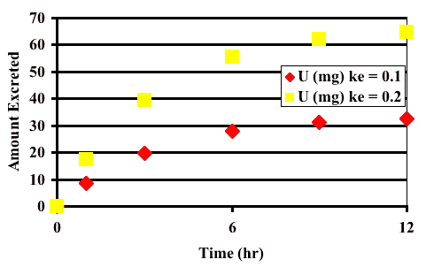
In both tables, above, the data calculated for Cp and Cm are identical even though quite different values of ke were used. The values of km and Vm were different to compensate but we can see that different values of ke could be determined from these data points. The only difference is in the U values. This indicates that a number of parameters including ke, km and Vm may not be identifiable when drug and metabolite concentration in blood or plasma are determined. However, collection of drug amounts in urine has the potential of making these parameters identifiable. This can be further illustrated by plotting these data.

Figure 20.3.3 Linear Plot of Cp and Cm versus Time with different values of ke

Figure 20.3.4 Linear Plot of U versus Time with different values of ke

Note that in Figure 20.3.3 there is only one line for Cp and Cm, respectively. In Figure 20.3.4 there are two lines for U for the two values of ke. If only Cp and cm are collected ke is non-identifiable and non-observable.

Dose Level Selection

Data collected after different dose levels can provide different information about pharmacokinetic parameters. This can lead to local non-identifiability. An example of this behavior can be seen with data collected (or simulated) with drugs which exhibit non-linear pharmacokinetics. In the simplest case the rate of elimination can be expressed using Michaelis-Menten parameters, Vmax and Km.

Equation 20.3.3 Rate of Elimination by Michaelis-Menten Kinetics

Figure 20.3.5 Semi-log Plot of Cp versus Time after Three Different Doses

In Figure 20.3.5 three lines are shown after three different doses. This is a semi-log plot. Note the lowest line appears to be a straight line looking like linear kinetics. It would be expected that only a kel value and not Vmax and Km values could be identified from this line of data points. The data collected at higher doses may be more useful in the determination of the Michaelis-Menten parameters. data from all three doses modeled simultaneously would be even better.

Sample Time Selection

Samples must be calculated at the best times to gain the best information about pharmacokinetic parameter values. The chapter on Optimal Sampling (Chapter 33) provides more information on determining the best time to sample to obtain good estimates of parameter values. For example if early data points are not available it can be difficult to determine good values of faster rate constants. The equation for drug concentration after oral administration contains to rate constants, kel and ka.

Equation 20.3.1 Drug concentration after Oral Administration

If ka is faster than kel then missing early time points can mean that the parameter ka is not locally identifiable. For example, if samples are only collected from four hours on as shown in Figure 20.3.6 ka will be poorly estimated.

Figure 20.3.6 Linear plot of Cp versus Time after Oral Administration

ka/kel Flip-Flop with Oral Dosing - Determining V and F

While analyzing concentration versus time data after oral administration we often assume that the absorption rate constant, ka, is larger than the elimination rate constant, kel. When using the method of residuals to estimate ka and kel we expect that ka is at least five times larger than kel. This is not always the case, especially with slow release dosage forms or drugs with rapid elimination. Given only oral dose concentration versus time data it is not possible to determine which is faster ka or kel. This is another example of global non-identifiable parmeters. Notice in Tables 20.3.3 and 20.3.4 the calculated concentrations are the same at each time point despite the differences in ka and kel values and the value for V. It should also be noted that with only oral data as presented in these two tables only a value for V/F is identifiable. Neither V or F can be determined. These identifiability problems can be easily solved with prior knowledge of the kel and F values from analysis of intravenous data or simultaneously analyzing iv and oral data at the same time.

Dose = 100 mg, ka = 1.0 hr^-1,
kel = 0.1 hr^-1, V = 10 L, F = 1
Time (hr)	Concentration (mg/L)
0	0.00
1	5.97
1.5	7.08
2	7.59
3	7.68
4	7.24
6	6.07
9	4.52
12	3.35
18	1.84
24	1.01

Table 20.3.3 Data after oral administration - ka > kel

Dose = 100 mg, ka = 0.1 hr^-1,
kel = 1.0 hr^-1, V = 1 L, F = 1
Time (hr)	Concentration (mg/L)
0	0.00
1	5.97
1.5	7.08
2	7.59
3	7.68
4	7.24
6	6.07
9	4.52
12	3.35
18	1.84
24	1.01

Table 20.3.4 Data after oral administration - ka < kel

This page describes a number of ways in which parameters may become non-identifiable and suggest ways of overcoming identifiability problems.

return to the Course index

This page was last modified: Sunday, 28th Jul 2024 at 5:04 pm

Privacy Statement - 25 May 2018

iBook and pdf versions of this material and other PK material is available