Chapter 5

Analysis of Urine Data

return to the Course index
previous | next

Example Calculation of Urine Analysis Plots

Table 5.6.1. Example Data Analysis of Drug in Urine Data

Time Interval (hr)	Urine Volume (ml)	Urine Concentration (mg/ml)	Amount Excreted ΔU (mg)	Cumulative Amount Excreted U (mg)	Midpoint Time tmidpt (hr)	Rate of Excretion ΔU/Δt (mg/hr)	A.R.E. (mg)
0 - 2	50	1.666	83.3	83.3			116.8
					1	41.7
2 - 4	46	1.069	49.2	132.5			67.7
					3	24.6
4 - 6	48	0.592	28.4	160.9			39.2
					5	14.2
6 - 8	49	0.335	16.4	177.3			22.8
					7	8.2
8 - 10	46	0.210	9.7	187			13.2
					9	4.8
10 - 12	48	0.116	5.6	192.5			7.6
					11	2.8
12 - 18	134	0.047	6.3	198.8			1.3
					15	1
18 - 24	144	0.009	1.3	200.1			-
					21	0.2
24 - ∞	-	-	-	200.1

Completing the Table

• Multiplying column 2 by column 3 gives column 4, the amount excreted during the interval, ΔU.
• Accumulating the ΔU amounts in column 4 gives the cumulative amount excreted, U, up to the end of the current time interval. The total amount excreted, U^∞ is found at the bottom of column 5, that is 200.1 mg.
• The rate of excretion, ΔU/Δt, is calculated by dividing the ΔU amount by the length of the time interval, Δt.
• A.R.E. in the last column is calculated by subtracting the value for U in each row from U^∞.

The Data Plots

Cumulative Amount Excreted into Urine Plot

Figure 5.6.1 Linear Plot of Cumulative Amount Excreted versus Time

The plot in Figure 5.6.1 shows U rapidly increasing at first then leveling off to U^∞ (= 200 mg). NOTE: U^∞ ≠ DOSE for this set of data. Notice that U^∞/2 (100 mg) is excreted in about 3 hours which gives an estimate of the elimination half-life. Otherwise this plot is a qualitative representation of the data.

Calculation Using Rate of Excretion Data

Figure 5.6.2 Semi-log Plot of Rate of Excretion versus Time

The plots in Figures 5.6.2 and 5.6.3 (below) are more useful for calculating parameter values. A straight line can be drawn through the data on each semi-log plot. The elimination rate constant, kel, can be determined from the slope of this line and ke or fe determined from the intercept.

Figure 5.6.2 provides a semi-log plot of ΔU/Δt versus t _midpoint. As you can see this gives a reasonably straight line plot.

Estimating the intercept value to be 53 mg/hr and if the line crosses the axis at 23.6 hr where the rate of excretion is 0.1 mg/hr a value for kel can be estimated.

and ke can be determined from the intercept.

Thus fe = ke/kel = 0.177/0.266 = 0.665.

This plot can be used to estimate kel, ke and fe. A disadvantage of this type of plot is that the error present in "real" data can obscure the straight line and lead to results which lack precision. Also it can be difficult to collect frequent, accurately timed urine samples. This is especially true when the elimination half-life is small.

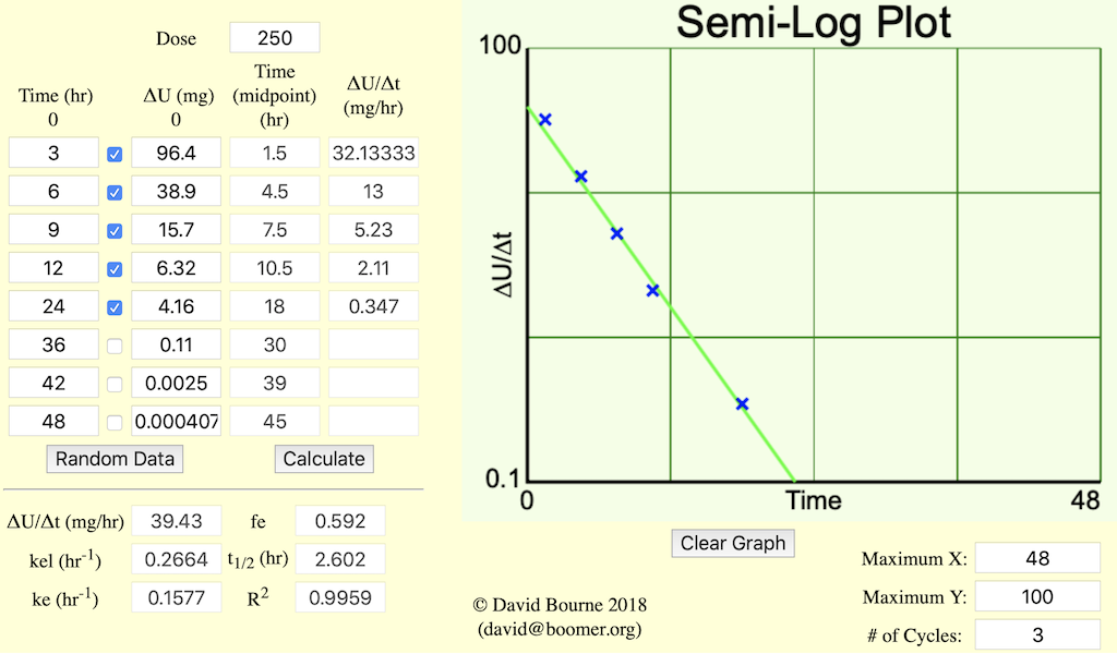
Figure 5.6.3 Analysis of Urine Data - Rate of Excretion

Calculation Using A.R.E. Data

Figure 5.6.4 Semi-log Plot of A.R.E. versus Time

The A.R.E. data are plotted as red circles on Figure 5.6.3 above. Estimating the intercept value to be 210 mg and if the line crosses the axis at 19 hr where the A.R.E. is 1 mg a value for kel can be estimated.

and fe can be determined from the intercept.

Thus ke = fe • kel = 0.7 x 0.281 = 0.197 hr^-1

One disadvantage of this approach is that the errors are cumulative, with collection interval, and the total error is incorporated into the U^∞ values and therefore into each A.R.E. value. Another problem is that total (all) urine collections are necessary. One missed sample means errors in all the results calculated.

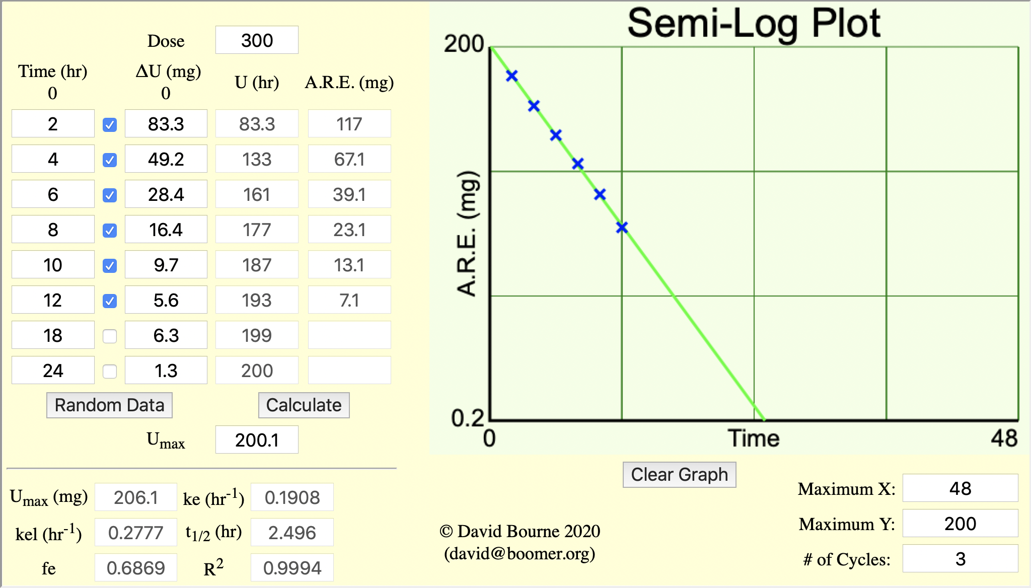
Figure 5.6.5 Analysis of Urine Data - Amount Remaining to Excreted

return to the Course index

Material on this website should be used for Educational or Self-Study Purposes Only

Copyright © 2001 - 2025 David W. A. Bourne (david@boomer.org)

Survey Help An iPhone app that allows the input of up to four locations (latitude and longitude) and provides the user's distance from each location